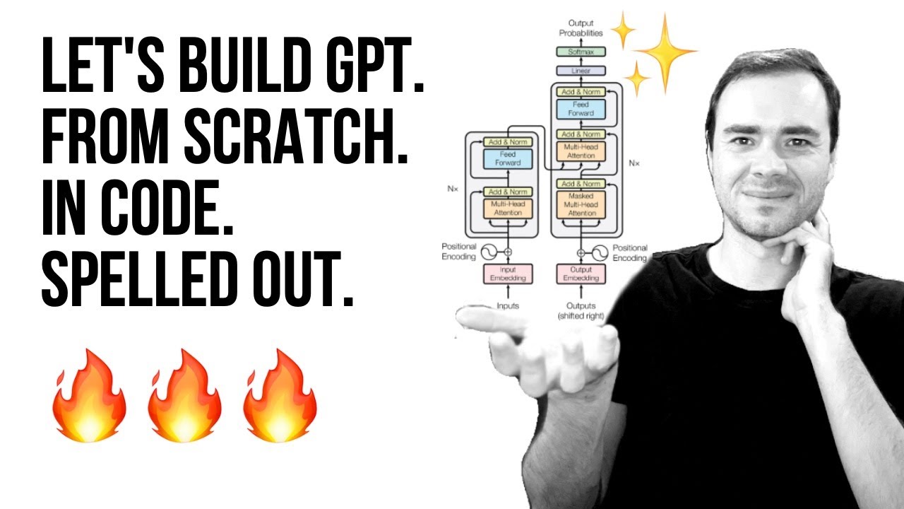
Let's build GPT: from scratch, in code, spelled out.
Now Playing
Let's build GPT: from scratch, in code, spelled out.
Transcript
2955 segments
hi everyone so by now you have probably
heard of chat GPT it has taken the world
and AI Community by storm and it is a
system that allows you to interact with
an AI and give it text based tasks so
for example we can ask chat GPT to write
us a small Hau about how important it is
that people understand Ai and then they
can use it to improve the world and make
it more prosperous so when we run this
AI knowledge brings prosperity for all
to see Embrace its
power okay not bad and so you could see
that chpt went from left to right and
generated all these words SE sort of
sequentially now I asked it already the
exact same prompt a little bit earlier
and it generated a slightly different
outcome ai's power to grow ignorance
holds us back learn Prosperity weights
so uh pretty good in both cases and
slightly different so you can see that
chat GPT is a probabilistic system and
for any one prompt it can give us
multiple answers sort of uh replying to
it now this is just one example of a
problem people have come up with many
many examples and there are entire
websites that index interactions with
chpt and so many of them are quite
humorous explain HTML to me like I'm a
dog uh write release notes for chess 2
write a note about Elon Musk buying a
Twitter and so on so as an example uh
please write a breaking news article
about a leaf falling from a
tree uh and a shocking turn of events a
leaf has fallen from a tree in the local
park Witnesses report that the leaf
which was previously attached to a
branch of a tree attached itself and
fell to the ground very dramatic so you
can see that this is a pretty remarkable
system and it is what we call a language
model uh because it um it models the
sequence of words or characters or
tokens more generally and it knows how
sort of words follow each other in
English language and so from its
perspective what it is doing is it is
completing the sequence so I give it the
start of a sequence and it completes the
sequence with the outcome and so it's a
language model in that sense now I would
like to focus on the under the hood of
um under the hood components of what
makes CH GPT work so what is the neural
network under the hood that models the
sequence of these words and that comes
from this paper called attention is all
you need in 2017 a landmark paper a
landmark paper in AI that produced and
proposed the Transformer
architecture so GPT is uh short for
generally generatively pre-trained
Transformer so Transformer is the neuron
nut that actually does all the heavy
lifting under the hood it comes from
this paper in 2017 now if you read this
paper this uh reads like a pretty random
machine translation paper and that's
because I think the authors didn't fully
anticipate the impact that the
Transformer would have on the field and
this architecture that they produced in
the context of machine translation in
their case actually ended up taking over
uh the rest of AI in the next 5 years
after and so this architecture with
minor changes was copy pasted into a
huge amount of applications in AI in
more recent years and that includes at
the core of chat GPT now we are not
going to what I'd like to do now is I'd
like to build out something like chat
GPT but uh we're not going to be able to
of course reproduce chat GPT this is a
very serious production grade system it
is trained on uh a good chunk of
internet and then there's a lot of uh
pre-training and fine-tuning stages to
it and so it's very complicated what I'd
like to focus on is just to train a
Transformer based language model and in
our case it's going to be a character
level language model I still think that
is uh very educational with respect to
how these systems work so I don't want
to train on the chunk of Internet we
need a smaller data set in this case I
propose that we work with uh my favorite
toy data set it's called tiny
Shakespeare and um what it is is
basically it's a concatenation of all of
the works of sh Shakespeare in my
understanding and so this is all of
Shakespeare in a single file uh this
file is about 1 megab and it's just all
of
Shakespeare and what we are going to do
now is we're going to basically model
how these characters uh follow each
other so for example given a chunk of
these characters like this uh given some
context of characters in the past the
Transformer neural network will look at
the characters that I've highlighted and
is going to predict that g is likely to
come next in the sequence and it's going
to do that because we're going to train
that Transformer on Shakespeare and it's
just going to try to produce uh
character sequences that look like this
and in that process is going to model
all the patterns inside this data so
once we've trained the system i' just
like to give you a preview we can
generate infinite Shakespeare and of
course it's a fake thing that looks kind
of like
Shakespeare
um apologies for there's some Jank that
I'm not able to resolve in in here but
um you can see how this is going
character by character and it's kind of
like predicting Shakespeare like
language so verily my Lord the sites
have left the again the king coming with
my curses with precious pale and then
tranos say something else Etc and this
is just coming out of the Transformer in
a very similar manner as it would come
out in chat GPT in our case character by
character in chat GPT uh it's coming out
on the token by token level and tokens
are these sort of like little subword
pieces so they're not Word level they're
kind of like word chunk
level um and now I've already written
this entire code uh to train these
Transformers um and it is in a GitHub
repository that you can find and it's
called nanog
GPT so nanog GPT is a repository that
you can find in my GitHub and it's a
repository for training Transformers um
on any given text and what I think is
interesting about it because there's
many ways to train Transformers but this
is a very simple implementation so it's
just two files of 300 lines of code each
one file defines the GPT model the
Transformer and one file trains it on
some given Text data set and here I'm
showing that if you train it on a open
web Text data set which is a fairly
large data set of web pages then I
reproduce the the performance of
gpt2 so gpt2 is an early version of open
AI GPT uh from 2017 if I recall
correctly and I've only so far
reproduced the the smallest 124 million
parameter model uh but basically this is
just proving that the codebase is
correctly arranged and I'm able to load
the uh neural network weights that openi
has released later so you can take a
look at the finished code here in N GPT
but what I would like to do in this
lecture is I would like to basically uh
write this repository from scratch so
we're going to begin with an empty file
and we're we're going to define a
Transformer piece by piece we're going
to train it on the tiny Shakespeare data
set and we'll see how we can then uh
generate infinite Shakespeare and of
course this can copy paste to any
arbitrary Text data set uh that you like
uh but my goal really here is to just
make you understand and appreciate uh
how under the hood chat GPT works and um
really all that's required is a
Proficiency in Python and uh some basic
understanding of um calculus and
statistics
and it would help if you also see my
previous videos on the same YouTube
channel in particular my make more
series where I um Define smaller and
simpler neural network language models
uh so multi perceptrons and so on it
really introduces the language modeling
framework and then uh here in this video
we're going to focus on the Transformer
neural network itself okay so I created
a new Google collab uh jup notebook here
and this will allow me to later easily
share this code that we're going to
develop together uh with you so you can
follow along so this will be in a video
description uh later now here I've just
done some preliminaries I downloaded the
data set the tiny Shakespeare data set
at this URL and you can see that it's
about a 1 Megabyte file then here I open
the input.txt file and just read in all
the text of the string and we see that
we are working with 1 million characters
roughly and the first 1,000 characters
if we just print them out are basically
what you would expect this is the first
1,000 characters of the tiny Shakespeare
data set roughly up to here so so far so
good next we're going to take this text
and the text is a sequence of characters
in Python so when I call the set
Constructor on it I'm just going to get
the set of all the characters that occur
in this text and then I call list on
that to create a list of those
characters instead of just a set so that
I have an ordering an arbitrary ordering
and then I sort that so basically we get
just all the characters that occur in
the entire data set and they're sorted
now the number of them is going to be
our vocabulary size these are the
possible elements of our sequences and
we see that when I print here the
characters there's 65 of them in total
there's a space character and then all
kinds of special characters and then U
capitals and lowercase letters so that's
our vocabulary and that's the sort of
like possible uh characters that the
model can see or emit okay so next we
will would like to develop some strategy
to tokenize the input text now when
people say tokenize they mean convert
the raw text as a string to some
sequence of integers According to some
uh notebook According to some vocabulary
of possible elements so as an example
here we are going to be building a
character level language model so we're
simply going to be translating
individual characters into integers so
let me show you uh a chunk of code that
sort of does that for us so we're
building both the encoder and the
decoder
and let me just talk through what's
happening
here when we encode an arbitrary text
like hi there we're going to receive a
list of integers that represents that
string so for example 46 47 Etc and then
we also have the reverse mapping so we
can take this list and decode it to get
back the exact same string so it's
really just like a translation to
integers and back for arbitrary string
and for us it is done on a character
level
now the way this was achieved is we just
iterate over all the characters here and
create a lookup table from the character
to the integer and vice versa and then
to encode some string we simply
translate all the characters
individually and to decode it back we
use the reverse mapping and concatenate
all of it now this is only one of many
possible encodings or many possible sort
of tokenizers and it's a very simple one
but there's many other schemas that
people have come up with in practice so
for example Google uses a sentence
piece uh so sentence piece will also
encode text into um integers but in a
different schema and using a different
vocabulary and sentence piece is a
subword uh sort of tokenizer and what
that means is that um you're not
encoding entire words but you're not
also encoding individual characters it's
it's a subword unit level and that's
usually what's adopted in practice for
example also openai has this Library
called tick token that uses a bite pair
encode
tokenizer um and that's what GPT uses
and you can also just encode words into
like hell world into a list of integers
so as an example I'm using the Tik token
Library here I'm getting the encoding
for gpt2 or that was used for gpt2
instead of just having 65 possible
characters or tokens they have 50,000
tokens and so when they encode the exact
same string High there we only get a
list of three integers but those
integers are not between 0 and 64 they
are between Z and 5,
5,256 so basically you can trade off the
code book size and the sequence lengths
so you can have very long sequences of
integers with very small vocabularies or
we can have short um sequences of
integers with very large vocabularies
and so typically people use in practice
these subword encodings but I'd like to
keep our token ier very simple so we're
using character level tokenizer and that
means that we have very small code books
we have very simple encode and decode
functions uh but we do get very long
sequences as a result but that's the
level at which we're going to stick with
this lecture because it's the simplest
thing okay so now that we have an
encoder and a decoder effectively a
tokenizer we can tokenize the entire
training set of Shakespeare so here's a
chunk of code that does that and I'm
going to start to use the pytorch
library and specifically the torch.
tensor from the pytorch library so we're
going to take all of the text in tiny
Shakespeare encode it and then wrap it
into a torch. tensor to get the data
tensor so here's what the data tensor
looks like when I look at just the first
1,000 characters or the 1,000 elements
of it so we see that we have a massive
sequence of integers and this sequence
of integers here is basically an
identical translation of the first
10,000 characters
here so I believe for example that zero
is a new line character and maybe one
one is a space not 100% sure but from
now on the entire data set of text is
re-represented as just it's just
stretched out as a single very large uh
sequence of
integers let me do one more thing before
we move on here I'd like to separate out
our data set into a train and a
validation split so in particular we're
going to take the first 90% of the data
set and consider that to be the training
data for the Transformer and we're going
to withhold the last 10% at the end of
it to be the validation data and this
will help us understand to what extent
our model is overfitting so we're going
to basically hide and keep the
validation data on the side because we
don't want just a perfect memorization
of this exact Shakespeare we want a
neural network that sort of creates
Shakespeare like uh text and so it
should be fairly likely for it to
produce the actual like stowed away uh
true Shakespeare text um and so we're
going to use this to uh get a sense of
the overfitting okay so now we would
like to start plugging these text
sequences or integer sequences into the
Transformer so that it can train and
learn those patterns now the important
thing to realize is we're never going to
actually feed entire text into a
Transformer all at once that would be
computationally very expensive and
prohibitive so when we actually train a
Transformer on a lot of these data sets
we only work with chunks of the data set
and when we train the Transformer we
basically sample random little chunks
out of the training set and train on
just chunks at a time and these chunks
have basically some kind of a length and
some maximum length now the maximum
length typically at least in the code I
usually write is called block size you
can you can uh find it under different
names like context length or something
like that let's start with the block
size of just eight and let me look at
the first train data characters the
first block size plus one characters
I'll explain why plus one in a
second so this is the first nine
characters in the sequence in the
training set now what I'd like to point
out is that when you sample a chunk of
data like this so say the these nine
characters out of the training set this
actually has multiple examples packed
into it and uh that's because all of
these characters follow each other and
so what this thing is going to say when
we plug it into a Transformer is we're
going to actually simultaneously train
it to make prediction at every one of
these
positions now in the in a chunk of nine
characters there's actually eight indiv
ual examples packed in there so there's
the example that when 18 when in the
context of 18 47 likely comes next in a
context of 18 and 47 56 comes next in a
context of 18 47 56 57 can come next and
so on so that's the eight individual
examples let me actually spell it out
with
code so here's a chunk of code to
illustrate X are the inputs to the
Transformer it will just be the first
block size characters y will be the uh
next block size characters so it's
offset by one and that's because y are
the targets for each position in the
input and then here I'm iterating over
all the block size of eight and the
context is always all the characters in
x uh up to T and including T and the
target is always the teth character but
in the targets array y so let me just
run
this and basically it spells out what I
said in words uh these are the eight
examples hidden in a chunk of nine
characters that we uh sampled from the
training set I want to mention one more
thing we train on all the eight examples
here with context between one all the
way up to context of block size and we
train on that not just for computational
reasons because we happen to have the
sequence already or something like that
it's not just done for efficiency it's
also done um to make the Transformer
Network be used to seeing contexts all
the way from as little as one all the
way to block size and we'd like the
transform to be used to seeing
everything in between and that's going
to be useful later during inference
because while we're sampling we can
start the sampling generation with as
little as one character of context and
the Transformer knows how to predict the
next character with all the way up to
just context of one and so then it can
predict everything up to block size and
after block size we have to start
truncating because the Transformer will
will never um receive more than block
size inputs when it's predicting the
next
character Okay so we've looked at the
time dimension of the tensors that are
going to be feeding into the Transformer
there's one more Dimension to care about
and that is the batch Dimension and so
as we're sampling these chunks of text
we're going to be actually every time
we're going to feed them into a
Transformer we're going to have many
batches of multiple chunks of text that
are all like stacked up in a single
tensor and that's just done for
efficiency just so that we can keep the
gpus busy uh because they are very good
at parallel processing of um of data and
so we just want to process multiple
chunks all at the same time but those
chunks are processed completely
independently they don't talk to each
other and so on so let me basically just
generalize this and introduce a batch
Dimension here's a chunk of
code let me just run it and then I'm
going to explain what it
does so here because we're going to
start sampling random locations in the
data set to pull chunks from I am
setting the seed so that um in the
random number generator so that the
numbers I see here are going to be the
same numbers you see later if you try to
reproduce this now the batch size here
is how many independent sequences we are
processing every forward backward pass
of the
Transformer the block size as I
explained is the maximum context length
to make those predictions so let's say B
size four block size eight and then
here's how we get batch for any
arbitrary split if the split is a
training split then we're going to look
at train data otherwise at valid data
that gives us the data array and then
when I Generate random positions to grab
a chunk out of I actually grab I
actually generate batch size number of
Random offsets so because this is four
we are ex is going to be a uh four
numbers that are randomly generated
between zero and Len of data minus block
size so it's just random offsets into
the training
set and then X's as I explained are the
first first block size characters
starting at I the Y's are the offset by
one of that so just add plus one and
then we're going to get those chunks for
every one of integers I INX and use a
torch. stack to take all those uh uh
one-dimensional tensors as we saw here
and we're going to um stack them up at
rows and so they all become a row in a
4x8 tensor
so here's where I'm printing then when I
sample a batch XB and YB the inputs to
the Transformer now are the input X is
the 4x8 tensor four uh rows of eight
columns and each one of these is a chunk
of the training
set and then the targets here are in the
associated array Y and they will come in
to the Transformer all the way at the
end uh to um create the loss function
uh so they will give us the correct
answer for every single position inside
X and then these are the four
independent
rows so spelled out as we did
before uh this 4x8 array contains a
total of 32 examples and they're
completely independent as far as the
Transformer is
concerned uh so when the input is 24 the
target is 43 or rather 43 here in the Y
array
when the input is 2443 the target is
58 uh when the input is 24 43 58 the
target is 5 Etc or like when it is a 52
581 the target is
58 right so you can sort of see this
spelled out these are the 32 independent
examples packed in to a single batch of
the input X and then the desired targets
are in y and so now this integer tensor
of um X is going to feed into the
Transformer and that Transformer is
going to simultaneously process all
these examples and then look up the
correct um integers to predict in every
one of these positions in the tensor y
okay so now that we have our batch of
input that we'd like to feed into a
Transformer let's start basically
feeding this into neural networks now
we're going to start off with the
simplest possible neural network which
in the case of language modeling in my
opinion is the Byram language model and
we've covered the Byram language model
in my make more series in a lot of depth
and so here I'm going to sort of go
faster and let's just Implement pytorch
module directly that implements the byr
language
model so I'm importing the pytorch um NN
module uh for
reproducibility and then here I'm
constructing a Byram language model
which is a subass of NN
module and then I'm calling it and I'm
passing it the inputs and the targets
and I'm just printing now when the
inputs on targets come here you see that
I'm just taking the index uh the inputs
X here which I rename to idx and I'm
just passing them into this token
embedding table so it's going on here is
that here in the Constructor we are
creating a token embedding table and it
is of size vocap size by vocap
size and we're using an. embedding which
is a very thin wrapper around basically
a tensor of shape voap size by vocab
size and what's happening here is that
when we pass idx here every single
integer in our input is going to refer
to this embedding table and it's going
to pluck out a row of that embedding
table corresponding to its index so 24
here will go into the embedding table
and we'll pluck out the 24th row and
then 43 will go here and pluck out the
43d row Etc and then pytorch is going to
arrange all of this into a batch by Time
by channel uh tensor in this case batch
is four time is eight and C which is the
channels is vocab size or 65 and so
we're just going to pluck out all those
rows arrange them in a b by T by C and
now we're going to interpret this as the
logits which are basically the scores
for the next character in the sequence
and so what's happening here is we are
predicting what comes next based on just
the individual identity of a single
token and you can do that because um I
mean currently the tokens are not
talking to each other and they're not
seeing any context except for they're
just seeing themselves so I'm a f I'm a
token number five and then I can
actually make pretty decent predictions
about what comes next just by knowing
that I'm token five because some
characters uh know um C follow other
characters in in typical scenarios so we
saw a lot of this in a lot more depth in
the make more series and here if I just
run this then we currently get the
predictions the scores the lits for
every one of the 4x8 positions now that
we've made predictions about what comes
next we'd like to evaluate the loss
function and so in make more series we
saw that a good way to measure a loss or
like a quality of the predictions is to
use the negative log likelihood loss
which is also implemented in pytorch
under the name cross entropy so what we'
like to do here is loss is the cross
entropy on the predictions and the
targets and so this measures the quality
of the logits with respect to the
Targets in other words we have the
identity of the next character so how
well are we predicting the next
character based on the lits and
intuitively the correct um the correct
dimension of low jits uh depending on
whatever the target is should have a
very high number and all the other
dimensions should be very low number
right now the issue is that this won't
actually this is what we want we want to
basically output the logits and the
loss this is what we want but
unfortunately uh this won't actually run
we get an error message but intuitively
we want to uh measure this now when we
go to the pytorch um cross entropy
documentation here um we're trying to
call the cross entropy in its functional
form uh so that means we don't have to
create like a module for it but here
when we go to the documentation you have
to look into the details of how pitor
expects these inputs and basically the
issue here is ptor expects if you have
multi-dimensional input which we do
because we have a b BYT by C tensor then
it actually really wants the channels to
be the second uh Dimension here so if
you um so basically it wants a b by C
BYT instead of a b by T by C and so it's
just the details of how P torch treats
um these kinds of inputs and so we don't
actually want to deal with that so what
we're going to do instead is we need to
basically reshape our logits so here's
what I like to do I like to take
basically give names to the dimensions
so lit. shape is B BYT by C and unpack
those numbers and then let's uh say that
logits equals lit. View and we want it
to be a b * c b * T by C so just a two-
dimensional
array right so we're going to take all
the we're going to take all of these um
positions here and we're going to uh
stretch them out in a onedimensional
sequence and uh preserve the channel
Dimension as the second
dimension so we're just kind of like
stretching out the array so it's two-
dimensional and in that case it's going
to better conform to what pytorch uh
sort of expects in its Dimensions now we
have to do the same to targets because
currently targets are um of shape B by T
and we want it to be just B * T so
onedimensional now alternatively you
could always still just do minus one
because pytor will guess what this
should be if you want to lay it out uh
but let me just be explicit and say p *
t once we've reshaped this it will match
the cross entropy case and then we
should be able to evaluate our
loss okay so that R now and we can do
loss and So currently we see that the
loss is
4.87 now because our uh we have 65
possible vocabulary elements we can
actually guess at what the loss should
be and in
particular we covered negative log
likelihood in a lot of detail we are
expecting log or lawn of um 1 over 65
and negative of that so we're expecting
the loss to be about 4.1 17 but we're
getting 4.87 and so that's telling us
that the initial predictions are not uh
super diffuse they've got a little bit
of entropy and so we're guessing wrong
uh so uh yes but actually we're I a we
are able to evaluate the loss okay so
now that we can evaluate the quality of
the model on some data we'd like to also
be able to generate from the model so
let's do the generation now I'm going to
go again a little bit faster here
because I covered all this already in
previous
videos
so here's a generate function for the
model so we take some uh we take the the
same kind of input idx here and
basically this is the current uh context
of some characters in a batch in some
batch so it's also B BYT and the job of
generate is to basically take this B BYT
and extend it to be B BYT + 1 plus 2
plus 3 and so it's just basically it
continues the generation in all the
batch dimensions in the time Dimension
So that's its job and it will do that
for Max new tokens so you can see here
on the bottom there's going to be some
stuff here but on the bottom whatever is
predicted is concatenated on top of the
previous idx along the First Dimension
which is the time Dimension to create a
b BYT + one so that becomes a new idx so
the job of generate is to take a b BYT
and make it a b BYT plus 1 plus 2 plus
three as many as we want Max new tokens
so this is the generation from the model
now inside the generation what what are
we doing we're taking the current
indices we're getting the predictions so
we get uh those are in the low jits and
then the loss here is going to be
ignored because um we're not we're not
using that and we have no targets that
are sort of ground truth targets that
we're going to be comparing with
then once we get the logits we are only
focusing on the last step so instead of
a b by T by C we're going to pluck out
the negative-1 the last element in the
time Dimension because those are the
predictions for what comes next so that
gives us the logits which we then
convert to probabilities via softmax and
then we use tor. multinomial to sample
from those probabilities and we ask
pytorch to give us one sample and so idx
next will become a b by one because in
each uh one of the batch Dimensions
we're going to have a single prediction
for what comes next so this num samples
equals one will make this be a
one and then we're going to take those
integers that come from the sampling
process according to the probability
distribution given here and those
integers got just concatenated on top of
the current sort of like running stream
of integers and this gives us a b BYT +
one and then we can return that now one
thing here is you see how I'm calling
self of idx which will end up going to
the forward function I'm not providing
any Targets So currently this would give
an error because targets is uh is uh
sort of like not given so targets has to
be optional so targets is none by
default and then if targets is none then
there's no loss to create so it's just
loss is none but else all of this
happens and we can create a loss so this
will make it so um if we have the
targets we provide them and get a loss
if we have no targets it will'll just
get the
loits so this here will generate from
the model um and let's take that for a
ride
now oops so I have another code chunk
here which will generate for the model
from the model and okay this is kind of
crazy so maybe let me let me break this
down so these are the idx
right I'm creating a batch will be just
one time will be just one so I'm
creating a little one by one tensor and
it's holding a zero and the D type the
data type is uh integer so zero is going
to be how we kick off the generation and
remember that zero is uh is the element
standing for a new line character so
it's kind of like a reasonable thing to
to feed in as the very first character
in a sequence to be the new
line um so it's going to be idx which
we're going to feed in here then we're
going to ask for 100 tokens
and then. generate will continue that
now because uh generate works on the
level of batches we we then have to
index into the zero throw to basically
unplug the um the single batch Dimension
that exists and then that gives us a um
time steps just a onedimensional array
of all the indices which we will convert
to simple python list from pytorch
tensor so that that can feed into our
decode function and uh convert those
integers into text so let me bring this
back and we're generating 100 tokens
let's
run and uh here's the generation that we
achieved so obviously it's garbage and
the reason it's garbage is because this
is a totally random model so next up
we're going to want to train this model
now one more thing I wanted to point out
here is this function is written to be
General but it's kind of like ridiculous
right now because
we're feeding in all this we're building
out this context and we're concatenating
it all and we're always feeding it all
into the model but that's kind of
ridiculous because this is just a simple
Byram model so to make for example this
prediction about K we only needed this W
but actually what we fed into the model
is we fed the entire sequence and then
we only looked at the very last piece
and predicted K so the only reason I'm
writing it in this way is because right
now this is a byr model but I'd like to
keep keep this function fixed and I'd
like it to work um later when our
characters actually um basically look
further in the history and so right now
the history is not used so this looks
silly uh but eventually the history will
be used and so that's why we want to uh
do it this way so just a quick comment
on that so now we see that this is um
random so let's train the model so it
becomes a bit less random okay let's Now
train the model so first what I'm going
to do is I'm going to create a pyour
optimization object so here we are using
the optimizer ATM W um now in a make
more series we've only ever use tastic
gradi in descent the simplest possible
Optimizer which you can get using the
SGD instead but I want to use Adam which
is a much more advanced and popular
Optimizer and it works extremely well
for uh typical good setting for the
learning rate is roughly 3 E4 uh but for
very very small networks like is the
case here you can get away with much
much higher learning rates R3 or even
higher probably but let me create the
optimizer object which will basically
take the gradients and uh update the
parameters using the
gradients and then here our batch size
up above was only four so let me
actually use something bigger let's say
32 and then for some number of steps um
we are sampling a new batch of data
we're evaluating the loss uh we're
zeroing out all the gradients from the
previous step getting the gradients for
all the parameters and then using those
gradients to up update our parameters so
typical training loop as we saw in the
make more series so let me now uh run
this for say 100 iterations and let's
see what kind of losses we're going to
get so we started around
4.7 and now we're getting to down to
like 4.6 4.5 Etc so the optimization is
definitely happening but um let's uh
sort of try to increase number of
iterations and only print at the
end because we probably want train for
longer okay so we're down to 3.6
roughly roughly down to
three this is the most janky
optimization okay it's working let's
just do
10,000 and then from here we want to
copy this and hopefully that we're going
to get something reason and of course
it's not going to be Shakespeare from a
byr model but at least we see that the
loss is improving and uh hopefully we're
expecting something a bit more
reasonable okay so we're down at about
2.5 is let's see what we get okay
dramatic improvements certainly on what
we had here so let me just increase the
number of tokens okay so we see that
we're starting to get something at least
like reasonable is
um certainly not shakes spear but uh the
model is making progress so that is the
simplest possible
model so now what I'd like to do
is obviously this is a very simple model
because the tokens are not talking to
each other so given the previous context
of whatever was generated we're only
looking at the very last character to
make the predictions about what comes
next so now these uh now these tokens
have to start talking to each other and
figuring out what is in the context so
that they can make better predictions
for what comes next and this is how
we're going to kick off the uh
Transformer okay so next I took the code
that we developed in this juper notebook
and I converted it to be a script and
I'm doing this because I just want to
simplify our intermediate work into just
the final product that we have at this
point so in the top here I put all the
hyp parameters that we to find I
introduced a few and I'm going to speak
to that in a little bit otherwise a lot
of this should be recognizable uh
reproducibility read data get the
encoder and the decoder create the train
into splits uh use the uh kind of like
data loader um that gets a batch of the
inputs and Targets this is new and I'll
talk about it in a second now this is
the Byram language model that we
developed and it can forward and give us
a logits and loss and it can
generate and then here we are creating
the optimizer and this is the training
Loop so everything here should look
pretty familiar now some of the small
things that I added number one I added
the ability to run on a GPU if you have
it so if you have a GPU then you can
this will use Cuda instead of just CPU
and everything will be a lot more faster
now when device becomes Cuda then we
need to make sure that when we load the
data we move it to
device when we create the model we want
to move uh the model parameters to
device so as an example here we have the
N an embedding table and it's got a
weight inside it which stores the uh
sort of lookup table so so that would be
moved to the GPU so that all the
calculations here happen on the GPU and
they can be a lot faster and then
finally here when I'm creating the
context that feeds in to generate I have
to make sure that I create it on the
device number two what I introduced is
uh the fact that here in the training
Loop here I was just printing the um l.
item inside the training Loop but this
is a very noisy measurement of the
current loss because every batch will be
more or less lucky and so what I want to
do usually um is uh I have an estimate
loss function and the estimate loss
basically then um goes up here and it
averages up the loss over multiple
batches so in particular we're going to
iterate eval iter times and we're going
to basically get our loss and then we're
going to get the average loss for both
splits and so this will be a lot less
noisy so here when we call the estimate
loss we're we're going to report the uh
pretty accurate train and validation
loss now when we come back up you'll
notice a few things here I'm setting the
model to evaluation phase and down here
I'm resetting it back to training phase
now right now for our model as is this
doesn't actually do anything because the
only thing inside this model is this uh
nn. embedding and um this this um
Network would behave both would behave
the same in both evaluation mode and
training mode we have no drop off layers
we have no batm layers Etc but it is a
good practice to Think Through what mode
your neural network is in because some
layers will have different Behavior Uh
at inference time or training time and
there's also this context manager torch
up nograd and this is just telling
pytorch that everything that happens
inside this function we will not call do
backward on and so pytorch can be a lot
more efficient with its memory use
because it doesn't have to store all the
intermediate variables uh because we're
never going to call backward and so it
can it can be a lot more memory
efficient in that way so also a good
practice to tpy torch when we don't
intend to do back
propagation so right now this script is
about 120 lines of code of and that's
kind of our starter code I'm calling it
b.p and I'm going to release it later
now running this
script gives us output in the terminal
and it looks something like this it
basically as I ran this code uh it was
giving me the train loss and Val loss
and we see that we convert to somewhere
around
2.5 with the pyr model and then here's
the sample that we produced at the
end and so we have everything packaged
up in the script and we're in a good
position now to iterate on this okay so
we are almost ready to start writing our
very first self attention block for
processing these uh tokens now before we
actually get there I want to get you
used to a mathematical trick that is
used in the self attention inside a
Transformer and is really just like at
the heart of an an efficient
implementation of self attention and so
I want to work with this toy example to
just get you used to this operation and
then it's going to make it much more
clear once we actually get to um to it
uh in the script
again so let's create a b BYT by C where
BT and C are just 48 and two in the toy
example and these are basically channels
and we have uh batches and we have the
time component and we have information
at each point in the sequence so
see now what we would like to do is we
would like these um tokens so we have up
to eight tokens here in a batch and
these eight tokens are currently not
talking to each other and we would like
them to talk to each other we'd like to
couple them and in particular we don't
we we want to couple them in a very
specific way so the token for example at
the fifth location it should not
communicate with tokens in the sixth
seventh and eighth location
because uh those are future tokens in
the sequence the token on the fifth
location should only talk to the one in
the fourth third second and first so
it's only so information only flows from
previous context to the current time
step and we cannot get any information
from the future because we are about to
try to predict the
future so what is the easiest way for
tokens to communicate okay the easiest
way I would say is okay if we're up to
if we're a fifth token and I'd like to
communicate with my past the simplest
way we can do that is to just do a
weight is to just do an average of all
the um of all the preceding elements so
for example if I'm the fif token I would
like to take the channels uh that make
up that are information at my step but
then also the channels from the fourth
step third step second step and the
first step I'd like to average those up
and then that would become sort of like
a feature Vector that summarizes me in
the context of my history now of course
just doing a sum or like an average is
an extremely weak form of interaction
like this communication is uh extremely
lossy we've lost a ton of information
about the spatial Arrangements of all
those tokens uh but that's okay for now
we'll see how we can bring that
information back later for now what we
would like to do is for every single
batch element independently for every
teeth token in that sequence we'd like
to now calculate the average of all the
vectors in all the previous tokens and
also at this token so let's write that
out um I have a small snippet here and
instead of just fumbling around let me
just copy paste it and talk to
it so in other words we're going to
create X and B is short for bag of words
because bag of words is um is kind of
like um a term that people use when you
are just averaging up things so this is
just a bag of words basically there's a
word stored on every one of these eight
locations and we're doing a bag of words
we're just averaging
so in the beginning we're going to say
that it's just initialized at Zero and
then I'm doing a for Loop here so we're
not being efficient yet that's coming
but for now we're just iterating over
all the batch Dimensions independently
iterating over time and then the
previous uh tokens are at this uh batch
Dimension and then everything up to and
including the teeth token okay so when
we slice out X in this way X prev
Becomes of shape um how many T elements
there were in the past and then of
course C so all the two-dimensional
information from these little tokens so
that's the previous uh sort of chunk of
um tokens from my current sequence and
then I'm just doing the average or the
mean over the zero Dimension so I'm
averaging out the time here and I'm just
going to get a little c one dimensional
Vector which I'm going to store in X bag
of words so I can run this and and uh
this is not going to be very informative
because let's see so this is X of Zer so
this is the zeroth batch element and
then expo at zero now you see how the at
the first location here you see that the
two are equal and that's because it's
we're just doing an average of this one
token but here this one is now an
average of these two and now this one is
an average of these
three and so on
so uh and this last one is the average
of all of these elements so vertical
average just averaging up all the tokens
now gives this outcome
here so this is all well and good uh but
this is very inefficient now the trick
is that we can be very very efficient
about doing this using matrix
multiplication so that's the
mathematical trick and let me show you
what I mean let's work with the toy
example here let me run it and I'll
explain I have a simple Matrix here that
is a 3X3 of all ones a matrix B of just
random numbers and it's a 3x2 and a
matrix C which will be 3x3 multip 3x2
which will give out a 3x2 so here we're
just using um matrix multiplication so a
multiply B gives us
C okay so how are these numbers in C um
achieved right so this number in the top
left is the first row of a dot product
with the First Column of B and since all
the the row of a right now is all just
ones then the do product here with with
this column of B is just going to do a
sum of these of this column so 2 + 6 + 6
is
14 the element here in the output of C
is also the first column here the first
row of a multiplied now with the second
column of B so 7 + 4 + 5 is 16 now you
see that there's repeating elements here
so this 14 again is because this row is
again all ones and it's multiplying the
First Column of B so we get 14 and this
one is and so on so this last number
here is the last row do product last
column now the trick here is uh the
following this is just a boring number
of um it's just a boring array of all
ones but torch has this function called
Trail which is short for a
triangular uh something like that and
you can wrap it in torch up once and it
will just return the lower triangular
portion of this
okay so now it will basically zero out
uh these guys here so we just get the
lower triangular part well what happens
if we do
that so now we'll have a like this and B
like this and now what are we getting
here in C well what is this number well
this is the first row times the First
Column and because this is zeros
uh these elements here are now ignored
so we just get a two and then this
number here is the first row times the
second column and because these are
zeros they get ignored and it's just
seven this seven multiplies this one but
look what happened here because this is
one and then zeros we what ended up
happening is we're just plucking out the
row of this row of B and that's what we
got now here we have one 1 Z so here 110
do product with these two columns will
now give us 2 + 6 which is 8 and 7 + 4
which is 11 and because this is 111 we
ended up with the addition of all of
them and so basically depending on how
many ones and zeros we have here we are
basically doing a sum currently of a
variable number of these rows and that
gets deposited into
C So currently we're doing sums because
these are ones but we can also do
average right and you can start to see
how we could do average uh of the rows
of B uh sort of in an incremental
fashion because we don't have to we can
basically normalize these rows so that
they sum to one and then we're going to
get an average so if we took a and then
we did aals
aide torch. sum in the um of a in the um
oneth Dimension and then let's keep them
as true so so therefore the broadcasting
will work out so if I rerun this you see
now that these rows now sum to one so
this row is one this row is 0. 5.5 Z and
here we get 1/3 and now when we do a
multiply B what are we getting here we
are just getting the first row first row
here now we are getting the average of
the first two
rows okay so 2 and six average is four
and four and seven average is
5.5 and on the bottom here we are now
getting the average of these three rows
so the average of all of elements of B
are now deposited here and so you can
see that by manipulating these uh
elements of this multiplying Matrix and
then multiplying it with any given
Matrix we can do these averages in this
incremental fashion because we just get
um and we can manipulate that based on
the elements of a okay so that's very
convenient so let's let's swing back up
here and see how we can vectorize this
and make it much more efficient using
what we've learned so in
particular we are going to produce an
array a but here I'm going to call it we
short for weights but this is our
a and this is how much of every row we
want to average up and it's going to be
an average because you can see that
these rows sum to
one so this is our a and then our B in
this example of course is X
so what's going to happen here now is
that we are going to have an expo
2 and this Expo 2 is going to be way
multiplying
RX so let's think this true way is T BYT
and this is Matrix multiplying in
pytorch a b by T by
C and it's giving us uh different what
shape so pytorch will come here and it
will see that these shapes are not the
same so it will create a batch Dimension
here and this is a batched matrix
multiply and so it will apply this
matrix multiplication in all the batch
elements um in parallel and individually
and then for each batch element there
will be a t BYT multiplying T by C
exactly as we had
below so this will now create B by T by
C and Expo 2 will now become identical
to Expo
so we can see that torch. all close of
xbo and xbo 2 should be true
now so this kind of like convinces us
that uh these are in fact um the same so
xbo and xbo 2 if I just print
them uh okay we're not going to be able
to okay we're not going to be able to
just stare it down but
um well let me try Expo basically just
at the zeroth element and Expo two at
the zeroth element so just the first
batch and we should see that this and
that should be identical which they
are right so what happened here the
trick is we were able to use batched
Matrix multiply to do this uh
aggregation really and it's a weighted
aggregation and the weights are
specified in this um T BYT array and
we're basically doing weighted sums and
uh these weighted sums are are U
according to uh the weights inside here
they take on sort of this triangular
form and so that means that a token at
the teth dimension will only get uh sort
of um information from the um tokens
perceiving it so that's exactly what we
want and finally I would like to rewrite
it in one more way and we're going to
see why that's useful so this is the
third version and it's also identical to
the first and second but let me talk
through it it uses
softmax so Trill here is this Matrix
lower triangular
ones way begins as all
zero okay so if I just print way in the
beginning it's all zero then I
used masked fill so what this is doing
is we. masked fill it's all zeros and
I'm saying for all the elements where
Trill is equal equal Z make them be
negative Infinity so all the elements
where Trill is zero will become negative
Infinity now so this is what we get and
then the final line here is
softmax so if I take a softmax along
every single so dim is negative one so
along every single row if I do softmax
what is that going to
do well softmax is um is also like a
normalization operation right and so
spoiler alert you get the exact same
Matrix let me bring back to
softmax and recall that in softmax we're
going to exponentiate every single one
of these and then we're going to divide
by the sum and so if we exponentiate
every single element here we're going to
get a one and here we're going to get uh
basically zero 0 z0 Z everywhere else
and then when we normalize we just get
one here we're going to get one one and
then zeros and then softmax will again
divide and this will give us 5.5 and so
on and so this is also the uh the same
way to produce uh this mask now the
reason that this is a bit more
interesting and the reason we're going
to end up using it in self
attention is that these weights here
begin uh with zero and you can think of
this as like an interaction strength or
like an affinity so basically it's
telling us how much of each uh token
from the past do we want to Aggregate
and average up
and then this line is saying tokens from
the past cannot communicate by setting
them to negative Infinity we're saying
that we will not aggregate anything from
those
tokens and so basically this then goes
through softmax and through the weighted
and this is the aggregation through
matrix
multiplication and so what this is now
is you can think of these as um these
zeros are currently just set by us to be
zero but a quick preview is that these
affinities between the tokens are not
going to be just constant at zero
they're going to be data dependent these
tokens are going to start looking at
each other and some tokens will find
other tokens more or less interesting
and depending on what their values are
they're going to find each other
interesting to different amounts and I'm
going to call those affinities I think
and then here we are saying the future
cannot communicate with the past we're
we're going to clamp them and then when
we normalize and sum we're going to
aggregate uh sort of their values
depending on how interesting they find
each other and so that's the preview for
self attention and basically long story
short from this entire section is that
you can do weighted aggregations of your
past
Elements by having by using matrix
multiplication of a lower triangular
fashion and then the elements here in
the lower triangular part are telling
you how much of each element uh fuses
into this position so we're going to use
this trick now to develop the self
attention block block so first let's get
some quick preliminaries out of the way
first the thing I'm kind of bothered by
is that you see how we're passing in
vocap size into the Constructor there's
no need to do that because vocap size is
already defined uh up top as a global
variable so there's no need to pass this
stuff
around next what I want to do is I don't
want to actually create I want to create
like a level of indirection here where
we don't directly go to the embedding
for the um logits but instead we go
through this intermediate phase because
we're going to start making that bigger
so let me introduce a new variable n
embed it shorted for number of embedding
Dimensions so
nbed here will be say 32 that was a
suggestion from GitHub co-pilot by the
way um it also suest 32 which is a good
number so this is an embedding table and
only 32 dimensional
embeddings so then here this is not
going to give us logits directly instead
this is going to give us token
embeddings that's I'm going to call it
and then to go from the token Tings to
the logits we're going to need a linear
layer so self. LM head let's call it
short for language modeling head is n
and linear from n ined up to vocap size
and then when we swing over here we're
actually going to get the loits by
exactly what the co-pilot says now we
have to be careful here because this C
and this C are not equal um this is nmed
C and this is vocap size so let's just
say that n ined is equal to
C and then this just creates one spous
layer of interaction through a linear
layer but uh this should basically
run so we see that this runs and uh this
currently looks kind of spous but uh
we're going to build on top of this now
next up so far we've taken these indices
and we've encoded them based on the
identity of the uh tokens in inside idx
the next thing that people very often do
is that we're not just encoding the
identity of these tokens but also their
position so we're going to have a second
position uh embedding table here so
self. position embedding table is an an
embedding of block size by an embed and
so each position from zero to block size
minus one will also get its own
embedding vector and then here first let
me decode B BYT from idx do
shape and then here we're also going to
have a pause embedding which is the
positional embedding and these are this
is to arrange so this will be basically
just integers from Z to T minus one and
all of those integers from 0 to T minus
one get embedded through the table to
create a t by
C and then here this gets renamed to
just say x and x will be the addition of
the token embeddings with the positional
embeddings and here the broadcasting
note will work out so B by T by C plus T
by C
this gets right aligned a new dimension
of one gets added and it gets
broadcasted across
batch so at this point x holds not just
the token identities but the positions
at which these tokens occur and this is
currently not that useful because of
course we just have a simple byr model
so it doesn't matter if you're in the
fifth position the second position or
wherever it's all translation invariant
at this stage uh so this information
currently wouldn't help uh but as we
work on the self attention block we'll
see that this starts to matter
okay so now we get the Crux of self
attention so this is probably the most
important part of this video to
understand we're going to implement a
small self attention for a single
individual head as they're called so we
start off with where we were so all of
this code is familiar so right now I'm
working with an example where I Chang
the number of channels from 2 to 32 so
we have a 4x8 arrangement of tokens and
each to and the information each token
is currently 32 dimensional but we just
are working with random
numbers now we saw here that the code as
we had it before does a uh simple weight
simple average of all the past tokens
and the current token so it's just the
previous information and current
information is just being mixed together
in an average and that's what this code
currently achieves and it Doo by
creating this lower triangular structure
which allows us to mask out this uh we
uh Matrix that we create so we mask it
out and then we normalize it and
currently when we initialize the
affinities between all the different
sort of tokens or nodes I'm going to use
those terms
interchangeably so when we initialize
the affinities between all the different
tokens to be zero then we see that way
gives us this um structure where every
single row has these um uniform numbers
and so that's what that's what then uh
in this Matrix multiply makes it so that
we're doing a simple
average now we don't actually want this
to be all uniform because different uh
tokens will find different other tokens
more or less interesting and we want
that to be data dependent so for example
if I'm a vowel then maybe I'm looking
for consonants in my past and maybe I
want to know what those consonants are
and I want that information to flow to
me and so I want to now gather
information from the past but I want to
do it in the data dependent way and this
is the problem that self attention
solves now the way self attention solves
this is the following every single node
or every single token at each position
will emit two vectors it will emit a
query and it will emit a
key now the query Vector roughly
speaking is what am I looking for and
the key Vector roughly speaking is what
do I
contain and then the way we get
affinities between these uh tokens now
in a sequence is we basically just do a
do product between the keys and the
queries so my query dot products with
all the keys of all the other tokens and
that dot product now becomes
wayy and so um if the key and the query
are sort of aligned they will interact
to a very high amount and then I will
get to learn more about that specific
token as opposed to any other token in
the sequence
so let's implement this
now we're going to implement a
single what's called head of self
attention so this is just one head
there's a hyper parameter involved with
these heads which is the head size and
then here I'm initializing linear
modules and I'm using bias equals false
so these are just going to apply a
matrix multiply with some fixed
weights and now let me produce a key and
q k and Q by forwarding these modules on
X so the size of this will now
become B by T by 16 because that is the
head size and the same here B by T by
16 so this being the head size so you
see here that when I forward this linear
on top of my X all the tokens in all the
positions in the B BYT Arrangement all
of them them in parallel and
independently produce a key and a query
so no communication has happened
yet but the communication comes now all
the queries will do product with all the
keys so basically what we want is we
want way now or the affinities between
these to be query multiplying key but we
have to be careful with uh we can't
Matrix multiply this we actually need to
transpose uh K but we have to be also
careful because these are when you have
The Bash Dimension so in particular we
want to transpose uh the last two
dimensions dimension1 and dimension -2
so
-21 and so this Matrix multiply now will
basically do the following B by T by
16 Matrix multiplies B by 16 by T to
give us B by T by
T right
so for every row of B we're now going to
have a t Square Matrix giving us the
affinities and these are now the way so
they're not zeros they are now coming
from this dot product between the keys
and the queries so this can now run I
can I can run this and the weighted
aggregation now is a function in a data
Bandon manner between the keys and
queries of these nodes so just
inspecting what happened
here the way takes on this form
and you see that before way was uh just
a constant so it was applied in the same
way to all the batch elements but now
every single batch elements will have
different sort of we because uh every
single batch element contains different
uh tokens at different positions and so
this is not data dependent so when we
look at just the zeroth uh Row for
example in the input these are the
weights that came out and so you can see
now that they're not just exactly
uniform um and in particular as an
example here for the last row this was
the eighth token and the eighth token
knows what content it has and it knows
at what position it's in and now the E
token based on that uh creates a query
hey I'm looking for this kind of stuff
um I'm a vowel I'm on the E position I'm
looking for any consonant at positions
up to four and then all the nodes get to
emit keys and maybe one of the channels
could be I am a I am a consonant and I
am in a position up to four and that
that key would have a high number in
that specific Channel and that's how the
query and the key when they do product
they can find each other and create a
high affinity and when they have a high
Affinity like say uh this token was
pretty interesting to uh to this eighth
token when they have a high Affinity
then through the softmax I will end up
aggregating a lot of its information
into my position and so I'll get to
learn a lot about
it now just this we're looking at way
after this has already happened um let
me erase this operation as well so let
me erase the masking and the softmax
just to show you the under the hood
internals and how that works so without
the masking in the softmax Whey comes
out like this right this is the outputs
of the do products um and these are the
raw outputs and they take on values from
negative you know two to positive two
Etc so that's the raw interactions and
raw affinities between all the nodes but
now if I'm going if I'm a fifth node I
will not want to aggregate anything from
the sixth node seventh node and the
eighth node so actually we use the upper
triangular masking so those are not
allowed to
communicate and now we actually want to
have a nice uh distribution uh so we
don't want to aggregate negative .11 of
this node that's crazy so instead we
exponentiate and normalize and now we
get a nice distribution that sums to one
and this is telling us now in the data
dependent manner how much of information
to aggregate from any of these tokens in
the
past so that's way and it's not zeros
anymore but but it's calculated in this
way now there's one more uh part to a
single self attention head and that is
that when we do the aggregation we don't
actually aggregate the tokens exactly we
aggregate we produce one more value here
and we call that the
value so in the same way that we
produced p and query we're also going to
create a value
and
then here we don't
aggregate X we calculate a v which is
just achieved by uh propagating this
linear on top of X again and then we
output way multiplied by V so V is the
elements that we aggregate or the the
vectors that we aggregate instead of the
raw
X and now of course uh this will make it
so that the output here of this single
head will be 16 dimensional because that
is the head
size so you can think of X as kind of
like private information to this token
if you if you think about it that way so
X is kind of private to this token so
I'm a fifth token at some and I have
some identity and uh my information is
kept in Vector X and now for the
purposes of the single head here's what
I'm interested in here's what I have and
if you find me interesting here's what I
will communicate to you and that's
stored in v and so V is the thing that
gets aggregated for the purposes of this
single head between the different
notes and that's uh basically the self
attention mechanism this is this is what
it does there are a few notes that I
would make like to make about attention
number one attention is a communication
mechanism you can really think about it
as a communication mechanism where you
have a number of nodes in a directed
graph where basically you have edges
pointed between noes like
this and what happens is every node has
some Vector of information and it gets
to aggregate information via a weighted
sum from all of the nodes that point to
it and this is done in a data dependent
manner so depending on whatever data is
actually stored that you should not at
any point in time now our graph doesn't
look like this our graph has a different
structure we have eight nodes because
the block size is eight and there's
always eight to
tokens and uh the first node is only
pointed to by itself the second node is
pointed to by the first node and itself
all the way up to the eighth node which
is pointed to by all the previous nodes
and itself and so that's the structure
that our directed graph has or happens
happens to have in Auto regressive sort
of scenario like language modeling but
in principle attention can be applied to
any arbitrary directed graph and it's
just a communication mechanism between
the nodes the second note is that notice
that there is no notion of space so
attention simply acts over like a set of
vectors in this graph and so by default
these nodes have no idea where they are
positioned in the space and that's why
we need to encode them positionally and
sort of give them some information that
is anchored to a specific position so
that they sort of know where they are
and this is different than for example
from convolution because if you're run
for example a convolution operation over
some input there's a very specific sort
of layout of the information in space
and the convolutional filters sort of
act in space and so it's it's not like
an attention in ATT ention is just a set
of vectors out there in space they
communicate and if you want them to have
a notion of space you need to
specifically add it which is what we've
done when we calculated the um relative
the positional encode encodings and
added that information to the vectors
the next thing that I hope is very clear
is that the elements across the batch
Dimension which are independent examples
never talk to each other they're always
processed independently and this is a
batched matrix multiply that applies
basically a matrix multiplication uh
kind of in parallel across the batch
dimension so maybe it would be more
accurate to say that in this analogy of
a directed graph we really have because
the back size is four we really have
four separate pools of eight nodes and
those eight nodes only talk to each
other but in total there's like 32 nodes
that are being processed uh but there's
um sort of four separate pools of eight
you can look at it that way the next
note is that here in the case of
language modeling uh we have this
specific uh structure of directed graph
where the future tokens will not
communicate to the Past tokens but this
doesn't necessarily have to be the
constraint in the general case and in
fact in many cases you may want to have
all of the uh noes talk to each other uh
fully so as an example if you're doing
sentiment analysis or something like
that with a Transformer you might have a
number of tokens and you may want to
have them all talk to each other fully
because later you are predicting for
example the sentiment of the sentence
and so it's okay for these NOS to talk
to each other and so in those cases you
will use an encoder block of self
attention and uh all it means that it's
an encoder block is that you will delete
this line of code allowing all the noes
to completely talk to each other what
we're implementing here is sometimes
called a decoder block and it's called a
decoder because it is sort of like a
decoding language and it's got this
autor regressive format where you have
to mask with the Triangular Matrix so
that uh nodes from the future never talk
to the Past because they would give away
the answer
and so basically in encoder blocks you
would delete this allow all the noes to
talk in decoder blocks this will always
be present so that you have this
triangular structure uh but both are
allowed and attention doesn't care
attention supports arbitrary
connectivity between nodes the next
thing I wanted to comment on is you keep
me you keep hearing me say attention
self attention Etc there's actually also
something called cross attention what is
the
difference
so basically the reason this attention
is self attention is because because the
keys queries and the values are all
coming from the same Source from X so
the same Source X produces Keys queries
and values so these nodes are self
attending but in principle attention is
much more General than that so for
example an encoder decoder Transformers
uh you can have a case where the queries
are produced from X but the keys and the
values come from a whole separate
external source and sometimes from uh
encoder blocks that encode some context
that we'd like to condition on
and so the keys and the values will
actually come from a whole separate
Source those are nodes on the side and
here we're just producing queries and
we're reading off information from the
side so cross attention is used when
there's a separate source of nodes we'd
like to pull information from into our
nodes and it's self attention if we just
have nodes that would like to look at
each other and talk to each other so
this attention here happens to be self
attention but in principle um attention
is a lot more General okay and the last
note at this stage is if we come to the
attention is all need paper here we've
already implemented attention so given
query key and value we've U multiplied
the query and a key we've soft maxed it
and then we are aggregating the values
there's one more thing that we're
missing here which is the dividing by
one / square root of the head size the
DK here is the head size why are they
doing this finds this important so they
call it the scaled attention and it's
kind of like an important normalization
to basically
have the problem is if you have unit gsh
and inputs so zero mean unit variance K
and Q are unit gashin then if you just
do we naively then you see that your we
actually will be uh the variance will be
on the order of head size which in our
case is 16 but if you multiply by one
over head size square root so this is
square root and this is one
over then the variance of we will be one
so it will be
preserved now why is this important
you'll not notice that way
here will feed into
softmax and so it's really important
especially at initialization that we be
fairly diffuse so in our case here we
sort of locked out here and we had a
fairly diffuse numbers here so um like
this now the problem is that because of
softmax if weight takes on very positive
and very negative numbers inside it
softmax will actually converge towards
one hot vectors and so I can illustrate
that here um say we are applying softmax
to a tensor of values that are very
close to zero then we're going to get a
diffuse thing out of
softmax but the moment I take the exact
same thing and I start sharpening it
making it bigger by multiplying these
numbers by eight for example you'll see
that the softmax will start to sharpen
and in fact it will sharpen towards the
max so it will sharpen towards whatever
number here is the highest and so um
basically we don't want these values to
be too extreme especially at
initialization otherwise softmax will be
way too peaky and um you're basically
aggregating um information from like a
single node every node just agregates
information from a single other node
that's not what we want especially at
initialization and so the scaling is
used just to control the variance at
initialization okay so having said all
that let's now take our self attention
knowledge and let's uh take it for a
spin so here in the code I created this
head module and it implements a single
head of self attention so you give it a
head size and then here it creates the
key query and the value linear layers
typically people don't use biases in
these uh so those are the linear
projections that we're going to apply to
all of our nodes now here I'm creating
this Trill variable Trill is not a
parameter of the module so in sort of
pytorch naming conventions uh this is
called a buffer it's not a parameter and
you have to call it you have to assign
it to the module using a register buffer
so that creates the trill uh the triang
lower triangular Matrix and we're given
the input X this should look very
familiar now we calculate the keys the
queries we C calculate the attention
scores inside way uh we normalize it so
we're using scaled attention here then
we make sure that uh future doesn't
communicate with the past so this makes
it a decoder block and then softmax and
then aggregate the value and
output then here in the language model
I'm creating a head in the Constructor
and I'm calling it self attention head
and the head size I'm going to keep as
the same and embed just for
now and then here once we've encoded the
information with the token embeddings
and the position embeddings we're simply
going to feed it into the self attention
head and then the output of that is
going to go into uh the decoder language
modeling head and create the logits so
this the sort of the simplest way to
plug in a self attention component uh
into our Network right now I had to make
one more change which is that here in
the generate uh we have to make sure
that our idx that we feed into the model
because now we're using positional
embeddings we can never have more than
block size coming in because if idx is
more than block size then our position
embedding table is going to run out of
scope because it only has embeddings for
up to block size and so therefore I
added some uh code here to crop the
context that we're going to feed into
self um so that uh we never pass in more
than block siiz elements
so those are the changes and let's Now
train the network okay so I also came up
to the script here and I decreased the
learning rate because uh the self
attention can't tolerate very very high
learning rates and then I also increased
number of iterations because the
learning rate is lower and then I
trained it and previously we were only
able to get to up to 2.5 and now we are
down to 2.4 so we definitely see a
little bit of an improvement from 2.5 to
2.4 roughly uh but the text is still not
amazing so clearly the self attention
head is doing some useful communication
but um we still have a long way to go
okay so now we've implemented the scale.
product attention now next up and the
attention is all you need paper there's
something called multi-head attention
and what is multi-head attention it's
just applying multiple attentions in
parallel and concatenating their results
so they have a little bit of diagram
here I don't know if this is super clear
it's really just multiple attentions in
parallel so let's Implement that fairly
straightforward
if we want a multi-head attention then
we want multiple heads of self attention
running in parallel so in pytorch we can
do this by simply creating multiple
heads so however heads how however many
heads you want and then what is the head
size of each and then we run all of them
in parallel into a list and simply
concatenate all of the outputs and we're
concatenating over the channel
Dimension so the way this looks now is
we don't have just a single ATT
that uh has a hit size of 32 because
remember n Ed is
32 instead of having one Communication
channel we now have four communication
channels in parallel and each one of
these communication channels typically
will be uh smaller uh correspondingly so
because we have four communication
channels we want eight dimensional self
attention and so from each Communication
channel we're going to together eight
dimensional vectors and then we have
four of them and that concatenates to
give us 32 which is the original and
embed and so this is kind of similar to
um if you're familiar with convolutions
this is kind of like a group convolution
uh because basically instead of having
one large convolution we do convolution
in groups and uh that's multi-headed
self
attention and so then here we just use
essay heads self attention heads instead
now I actually ran it and uh scrolling
down I ran the same thing and then we
now get this down to 2.28 roughly and
the output is still the generation is
still not amazing but clearly the
validation loss is improving because we
were at 2.4 just now and so it helps to
have multiple communication channels
because obviously these tokens have a
lot to talk about they want to find the
consonants the vowels they want to find
the vowels just from certain positions
uh they want to find any kinds of
different things and so it helps to
create multiple independent channels of
communication gather lots of different
types of data and then uh decode the
output now going back to the paper for a
second of course I didn't explain this
figure in full detail but we are
starting to see some components of what
we've already implemented we have the
positional encodings the token encodings
that add we have the masked multi-headed
attention implemented now here's another
multi-headed attention which is a cross
attention to an encoder which we haven't
we're not going to implement in this
case I'm going to come back to that
later but I want you to notice that
there's a feed forward part here and
then this is grouped into a block that
gets repeat it again and again now the
feedforward part here is just a simple
uh multi-layer perceptron
um so the multi-headed so here position
wise feed forward networks is just a
simple little MLP so I want to start
basically in a similar fashion also
adding computation into the network and
this computation is on a per node level
so I've already implemented it and you
can see the diff highlighted on the left
here when I've added or changed things
now before we had the self multi-headed
self attention that did the
communication but we went way too fast
to calculate the logits so the tokens
looked at each other but didn't really
have a lot of time to think on what they
found from the other tokens and so what
I've implemented here is a little feet
forward single layer and this little
layer is just a linear followed by a Rel
nonlinearity and that's that's it so
it's just a little layer and then I call
it feed
forward um and embed
and then this feed forward is just
called sequentially right after the self
attention so we self attend then we feed
forward and you'll notice that the feet
forward here when it's applying linear
this is on a per token level all the
tokens do this independently so the self
attention is the communication and then
once they've gathered all the data now
they need to think on that data
individually and so that's what feed
forward is doing and that's why I've
added it here now when I train this the
validation LW actually continues to go
down now to 2. 24 which is down from
2.28 uh the output still look kind of
terrible but at least we've improved the
situation and so as a preview we're
going to now start to intersperse the
communication with the computation and
that's also what the Transformer does
when it has blocks that communicate and
then compute and it groups them and
replicates them okay so let me show you
what we'd like to do we'd like to do
something like this we have a block and
this block is is basically this part
here except for the cross
attention now the block basically
intersperses communication and then
computation the computation the
communication is done using multi-headed
selfelf attention and then the
computation is done using a feed forward
Network on all the tokens
independently now what I've added here
also is you'll
notice this takes the number of
embeddings in the embedding Dimension
and number of heads that we would like
which is kind of like group size in
group convolution and and I'm saying
that number of heads we'd like is four
and so because this is 32 we calculate
that because this is 32 the number of
heads should be four um the head size
should be eight so that everything sort
of works out Channel wise um so this is
how the Transformer structures uh sort
of the uh the sizes typically so the
head size will become eight and then
this is how we want to intersperse them
and then here I'm trying to create
blocks which is just a sequential
application of block block block so that
we're interspersing communication feed
forward many many times and then finally
we decode now I actually tried to run
this and the problem is this doesn't
actually give a very good uh answer and
very good result and the reason for that
is we're start starting to actually get
like a pretty deep neural net and deep
neural Nets uh suffer from optimization
issues and I think that's what we're
kind of like slightly starting to run
into so we need one more idea that we
can borrow from the um Transformer paper
to resolve those difficulties now there
are two optimizations that dramatically
help with the depth of these networks
and make sure that the networks remain
optimizable let's talk about the first
one the first one in this diagram is you
see this Arrow here and then this arrow
and this Arrow those are skip
connections or sometimes called residual
connections they come from this paper uh
the presidual learning for image
recognition from about
2015 uh that introduced the concept now
these are basically what it means is you
transform data but then you have a skip
connection with addition from the
previous features now the way I like to
visualize it uh that I prefer is the
following here the computation happens
from the top to bottom and basically you
have this uh residual pathway and you
are free to Fork off from the residual
pathway perform some computation and
then project back to the residual
pathway via addition and so you go from
the the uh inputs to the targets only
via plus and plus plus and the reason
this is useful is because during back
propagation remember from our microG
grad video earlier addition distributes
gradients equally to both of its
branches that that fed as the input and
so the supervision or the gradients from
the loss basically hop through every
addition node all the way to the input
and then also Fork off into the residual
blocks but basically you have this
gradient Super Highway that goes
directly from the supervision all the
way to the input unimpeded and then
these viral blocks are usually
initialized in the beginning so they
contribute very very little if anything
to the residual pathway they they are
initialized that way so in the beginning
they are sort of almost kind of like not
there but then during the optimization
they come online over time and they uh
start to contribute but at least at the
initialization you can go from directly
supervision to the input gradient is
unimpeded and just flows and then the
blocks over time
kick in and so that dramatically helps
with the optimization so let's implement
this so coming back to our block here
basically what we want to do is we want
to do xal
X+ self attention and xal X+ self. feed
forward so this is X and then we Fork
off and do some communication and come
back and we Fork off and we do some
computation and come back so those are
residual connections and then swinging
back up here we also have to introd use
this projection so nn.
linear and uh this is going to be
from after we concatenate this this is
the prze and embed so this is the output
of the self tension itself but then we
actually want the uh to apply the
projection and that's the
result so the projection is just a
linear transformation of the outcome of
this
layer so that's the projection back into
the virual pathway and then here in a
feet forward it's going to be the same
same thing I could have a a self doot
projection here as well but let me just
simplify it and let me uh couple it
inside the same sequential container and
so this is the projection layer going
back into the residual
pathway and
so that's uh well that's it so now we
can train this so I implemented one more
small change when you look into the
paper again you see that the
dimensionality of input and output is
512 for them and they're saying that the
inner layer here in the feet forward has
dimensionality of 248 so there's a
multiplier of four and so the inner
layer of the feet forward Network should
be multiplied by four in terms of
Channel sizes so I came here and I
multiplied four times embed here for the
feed forward and then from four times
nmed coming back down to nmed when we go
back to the pro uh to the projection so
adding a bit of computation here and
growing that layer that is in the
residual block on the side of the
residual
pathway and then I train this and we
actually get down all the way to uh 2.08
validation loss and we also see that
network is starting to get big enough
that our train loss is getting ahead of
validation loss so we're starting to see
like a little bit of
overfitting and um our our
um uh Generations here are still not
amazing but at least you see that we can
see like is here this now grief syn like
this starts to almost look like English
so um yeah we're starting to really get
there okay and the second Innovation
that is very helpful for optimizing very
deep neural networks is right here so we
have this addition now that's the
residual part but this Norm is referring
to something called layer Norm so layer
Norm is implemented in pytorch it's a
paper that came out a while back here
um and layer Norm is very very similar
to bash Norm so remember back to our
make more series part three we
implemented bash
normalization and uh bash normalization
basically just made sure that um Across
The Bash dimension any individual neuron
had unit uh Gan um distribution so it
was zero mean and unit standard
deviation one standard deviation output
so what I did here is I'm copy pasting
the bashor 1D that we developed in our
make more series and see here we can
initialize for example this module and
we can have a batch of 32 100
dimensional vectors feeding through the
bachor layer so what this does is it
guarantees that when we look at just the
zeroth column it's a zero mean one
standard deviation so it's normalizing
every single column of this uh input now
the rows are not uh going to be
normalized by default because we're just
normalizing columns so let's now
Implement layer Norm uh it's very
complicated look we come here we change
this from zero to one so we don't
normalize The Columns we normalize the
rows and now we've implemented layer
Norm
so now the columns are not going to be
normalized um but the rows are going to
be normalized for every individual
example it's 100 dimensional Vector is
normalized uh in this way and because
our computation Now does not span across
examples we can delete all of this
buffers stuff uh because uh we can
always apply this operation and don't
need to maintain any running buffers so
we don't need the
buffers uh we
don't There's no distinction between
training and test
time uh and we don't need these running
buffers we do keep gamma and beta we
don't need the momentum we don't care if
it's training or not and this is now a
layer
norm and it normalizes the rows instead
of the columns and this here is
identical to basically this here so
let's now Implement layer Norm in our
Transformer before I incorporate the
layer Norm I just wanted to note that as
I said very few details about the
Transformer have changed in the last 5
years but this is actually something
that slightly departs from the original
paper you see that the ADD and Norm is
applied after the
transformation but um in now it is a bit
more uh basically common to apply the
layer Norm before the transformation so
there's a reshuffling of the layer Norms
uh so this is called the prorm
formulation and that's the one that
we're going to implement as well so
select deviation from the original paper
basically we need two layer Norms layer
Norm one is uh NN do layer norm and we
tell it how many um what is the
embedding Dimension and we need the
second layer norm and then here the
layer Norms are applied immediately on X
so self. layer Norm one applied on X and
self. layer Norm two applied on X before
it goes into self attention and feed
forward and uh the size of the layer
Norm here is an ed so 32 so when the
layer Norm is normalizing our features
it is uh the normalization here uh
happens the mean and the variance are
taken over 32 numbers so the batch and
the time act as batch Dimensions both of
them so this is kind of like a per token
um transformation that just normalizes
the features and makes them a unit mean
uh unit Gan at
initialization but of course because
these layer Norms inside it have these
gamma and beta training
parameters uh the layer Norm will U
eventually create outputs that might not
be unit gion but the optimization will
determine that so for now this is the uh
this is incorporating the layer norms
and let's train them on okay so I let it
run and we see that we get down to 2.06
which is better than the previous 2.08
so a slight Improvement by adding the
layer norms and I'd expect that they
help uh even more if we had bigger and
deeper Network one more thing I forgot
to add is that there should be a layer
Norm here also typically as at the end
of the Transformer and right before the
final uh linear layer that decodes into
vocabulary so I added that as well so at
this stage we actually have a pretty
complete uh Transformer according to the
original paper and it's a decoder only
Transformer I'll I'll talk about that in
a second uh but at this stage uh the
major pieces are in place so we can try
to scale this up and see how well we can
push this number now in order to scale
out the model I had to perform some
cosmetic changes here to make it nicer
so I introduced this variable called n
layer which just specifies how many
layers of the blocks we're going to have
I created a bunch of blocks and we have
a new variable number of heads as well I
pulled out the layer Norm here and uh so
this is identical now one thing that I
did briefly change is I added a Dropout
so Dropout is something that you can add
right before the residual connection
back right before the connection back
into the residual pathway so we can drop
out that as l layer here we can drop out
uh here at the end of the multi-headed
exension as well and we can also drop
out here uh when we calculate the um
basically affinities and after the
softmax we can drop out some of those so
we can randomly prevent some of the
nodes from
communicating and so Dropout uh comes
from this paper from 2014 or so and
basically it takes your neural
nut and it randomly every forward
backward pass shuts off some subset of
uh neurons so randomly drops them to
zero and trains without them and what
this does effectively is because the
mask of what's being dropped out is
changed every single forward backward
pass it ends up kind of uh training an
ensemble of sub networks and then at
test time everything is fully enabled
and kind of all of those sub networks
are merged into a single Ensemble if you
can if you want to think about it that
way so I would read the paper to get the
full detail for now we're just going to
stay on the level of this is a
regularization technique and I added it
because I'm about to scale up the model
quite a bit and I was concerned about
overfitting so now when we scroll up to
the top uh we'll see that I changed a
number of hyper parameters here about
our neural nut so I made the batch size
be much larger now it's 64 I changed the
block size to be 256 so previously it
was just eight eight characters of
context now it is 256 characters of
context to predict the 257th
uh I brought down the learning rate a
little bit because the neural net is now
much bigger so I brought down the
learning rate the embedding Dimension is
now 384 and there are six heads so 384
divide 6 means that every head is 64
dimensional as it as a standard and then
there's going to be six layers of that
and the Dropout will be at 02 so every
forward backward pass 20% of all of
these um intermediate calculations are
disabled and dropped to zero
and then I already trained this and I
ran it so uh drum roll how well does it
perform so let me just scroll up
here we get a validation loss of
1.48 which is actually quite a bit of an
improvement on what we had before which
I think was 2.07 so it went from 2.07
all the way down to 1.48 just by scaling
up this neural nut with the code that we
have and this of course ran for a lot
longer this maybe trained for I want to
say about 15 minutes on my a100 GPU so
that's a pretty a GPU and if you don't
have a GPU you're not going to be able
to reproduce this uh on a CPU this would
be um I would not run this on a CPU or
MacBook or something like that you'll
have to Brak down the number of uh
layers and the embedding Dimension and
so on uh but in about 15 minutes we can
get this kind of a result and um I'm
printing some of the Shakespeare here
but what I did also is I printed 10,000
characters so a lot more and I wrote
them to a file and so here we see some
of the outputs
so it's a lot more recognizable as the
input text file so the input text file
just for reference looked like this so
there's always like someone speaking in
this manner and uh our predictions now
take on that form except of course
they're they're nonsensical when you
actually read them
so it is every crimp tap be a house oh
those
prepation we give
heed um you know
Oho sent me you mighty
Lord anyway so you can read through this
um it's nonsensical of course but this
is just a Transformer trained on a
character level for 1 million characters
that come from Shakespeare so there's
sort of like blabbers on in Shakespeare
like manner but it doesn't of course
make sense at this scale uh but I think
I think still a pretty good
demonstration of what's
possible so now
I think uh that kind of like concludes
the programming section of this video we
basically kind of uh did a pretty good
job and um of implementing this
Transformer uh but the picture doesn't
exactly match up to what we've done so
what's going on with all these digital
Parts here so let me finish explaining
this architecture and why it looks so
funky basically what's happening here is
what we implemented here is a decoder
only Transformer so there's no component
here this part is called the encoder and
there's no cross attention block here
our block only has a self attention and
the feet forward so it is missing this
third in between piece here this piece
does cross attention so we don't have it
and we don't have the encoder we just
have the decoder and the reason we have
a decoder only uh is because we are just
uh generating text and it's
unconditioned on anything we're just
we're just blabbering on according to a
given data set what makes it a decoder
is that we are using the Triangular mask
in our uh trans former so it has this
Auto regressive property where we can
just uh go and sample from it so the
fact that it's using the Triangular
triangular mask to mask out the
attention makes it a decoder and it can
be used for language modeling now the
reason that the original paper had an
incoder decoder architecture is because
it is a machine translation paper so it
is concerned with a different setting in
particular it expects some uh tokens
that encode say for example French and
then it is expecting to decode the
translation in English so so you
typically these here are special tokens
so you are expected to read in this and
condition on it and then you start off
the generation with a special token
called start so this is a special new
token um that you introduce and always
place in the beginning and then the
network is expected to Output neural
networks are awesome and then a special
end token to finish the
generation so this part here will be
decoded exactly as we we've done it
neural networks are awesome will be
identical to what we did but unlike what
we did they wanton to condition the
generation on some additional
information and in that case this
additional information is the French
sentence that they should be
translating so what they do now is they
bring in the encoder now the encoder
reads this part here so we're only going
to take the part of French and we're
going to uh create tokens from it
exactly as we've seen in our video and
we're going to put a Transformer on it
but there's going to be no triangular
mask and so all the tokens are allowed
to talk to each other as much as they
want and they're just encoding
whatever's the content of this French uh
sentence once they've encoded it they
they basically come out in the top here
and then what happens here is in our
decoder which does the uh language
modeling there's an additional
connection here to the outputs of the
encoder
and that is brought in through a cross
attention so the queries are still
generated from X but now the keys and
the values are coming from the side the
keys and the values are coming from the
top generated by the nodes that came
outside of the de the encoder and those
tops the keys and the values there the
top of it feed in on a side into every
single block of the decoder and so
that's why there's an additional cross
attention and really what it's doing is
it's conditioning the decoding
not just on the past of this current
decoding but also on having seen the
full fully encoded French um prompt sort
of and so it's an encoder decoder model
which is why we have those two
Transformers an additional block and so
on so we did not do this because we have
no we have nothing to encode there's no
conditioning we just have a text file
and we just want to imitate it and
that's why we are using a decoder only
Transformer exactly as done in
GPT okay okay so now I wanted to do a
very brief walkthrough of nanog GPT
which you can find in my GitHub and uh
nanog GPT is basically two files of
Interest there's train.py and model.py
train.py is all the boilerplate code for
training the network it is basically all
the stuff that we had here it's the
training loop it's just that it's a lot
more complicated because we're saving
and loading checkpoints and pre-trained
weights and we are uh decaying the
learning rate and compiling the model
and using distributed training across
multiple nodes or GP use so the training
Pi gets a little bit more hairy
complicated uh there's more options Etc
but the model.py should look very very
um similar to what we've done here in
fact the model is is almost identical so
first here we have the causal self
attention block and all of this should
look very very recognizable to you we're
producing queries Keys values we're
doing Dot products we're masking
applying soft Maxs optionally dropping
out and here we are pulling the wi the
values what is different here is that in
our code I have separated out the
multi-headed detention into just a
single individual head and then here I
have multiple heads and I explicitly
concatenate them whereas here uh all of
it is implemented in a batched manner
inside a single causal self attention
and so we don't just have a b and a T
and A C Dimension we also end up with a
fourth dimension which is the heads and
so it just gets a lot more sort of hairy
because we have four dimensional array
um tensors now but it is um equivalent
mathematically so the exact same thing
is happening as what we have it's just
it's a bit more efficient because all
the heads are now treated as a batch
Dimension as
well then we have the multier perceptron
it's using the Galu nonlinearity which
is defined here except instead of Ru and
this is done just because opening I used
it and I want to be able to load their
checkpoints uh the blocks of the
Transformer are identical to communicate
in the compute phase as we saw and then
the GPT will be identical we have the
position encodings token encodings the
blocks the layer Norm at the end uh the
final linear layer and this should look
all very recognizable and there's a bit
more here because I'm loading
checkpoints and stuff like that I'm
separating out the parameters into those
that should be weight decayed and those
that
shouldn't um but the generate function
should also be very very similar so a
few details are different but you should
definitely be able to look at this uh
file and be able to understand little
the pieces now so let's now bring things
back to chat GPT what would it look like
if we wanted to train chat GPT ourselves
and how does it relate to what we
learned today well to train in chat GPT
there are roughly two stages first is
the pre-training stage and then the
fine-tuning stage in the pre-training
stage uh we are training on a large
chunk of internet and just trying to get
a first decoder only Transformer to
babble text so it's very very similar to
what we've done ourselves except we've
done like a tiny little baby
pre-training step um and so in our case
uh this is how you print a number of
parameters I printed it and it's about
10 million so this Transformer that I
created here to create little
Shakespeare um Transformer was about 10
million parameters our data set is
roughly 1 million uh characters so
roughly 1 million tokens but you have to
remember that opening I is different
vocabulary they're not on the Character
level they use these um subword chunks
of words and so they have a vocabulary
of 50,000 roughly elements and so their
sequences are a bit more condensed so
our data set the Shakespeare data set
would be probably around 300,000 uh
tokens in the open AI vocabulary roughly
so we trained about 10 million parameter
model on roughly 300,000 tokens now when
you go to the gpt3
paper and you look at the Transformers
that they trained they trained a number
of trans Transformers of different sizes
but the biggest Transformer here has 175
billion parameters uh so ours is again
10 million they used this number of
layers in the Transformer this is the
nmed this is the number of heads and
this is the head size and then this is
the batch size uh so ours was
65 and the learning rate is similar now
when they train this Transformer they
trained on 300 billion tokens so again
remember ours is about 300,000
so this is uh about a millionfold
increase and this number would not be
even that large by today's standards
you'd be going up uh 1 trillion and
above so they are training a
significantly larger
model on uh a good chunk of the internet
and that is the pre-training stage but
otherwise these hyper parameters should
be fairly recognizable to you and the
architecture is actually like nearly
identical to what we implemented
ourselves but of course it's a massive
infrastructure challenge to train this
you're talking about typically thousands
of gpus having to you know talk to each
other to train models of this size so
that's just a pre-training stage now
after you complete the pre-training
stage uh you don't get something that
responds to your questions with answers
and is not helpful and Etc you get a
document
completer right so it babbles but it
doesn't Babble Shakespeare it babbles
internet it will create arbitrary news
articles and documents and it will try
to complete documents because that's
what it's trained for it's trying to
complete the sequence so when you give
it a question it would just uh
potentially just give you more questions
it would follow with more questions it
will do whatever it looks like the some
close document would do in the training
data on the internet and so who knows
you're getting kind of like undefined
Behavior it might basically answer with
to questions with other questions it
might ignore your question it might just
try to complete some news article it's
totally unineed as we say so the second
fine-tuning stage is to actually align
it to be an assistant and uh this is the
second stage and so this chat GPT block
post from openi talks a little bit about
how the stage is achieved we basically
um there's roughly three steps to to
this stage uh so what they do here is
they start to collect training data that
looks specifically like what an
assistant would do so these are
documents that have to format where the
question is on top and then an answer is
below and they have a large number of
these but probably not on the order of
the internet uh this is probably on the
of maybe thousands of examples and so
they they then fine-tune the model to
basically only focus on documents that
look like that and so you're starting to
slowly align it so it's going to expect
a question at the top and it's going to
expect to complete the answer and uh
these very very large models are very
sample efficient during their
fine-tuning so this actually somehow
works but that's just step one that's
just fine tuning so then they actually
have more steps where okay the second
step is you let the model respond and
then different Raiders look at the
different responses and rank them for
their preference as to which one is
better than the other they use that to
train a reward model so they can predict
uh basically using a different network
how much of any candidate
response would be desirable and then
once they have a reward model they run
po which is a form of polic policy
gradient um reinforcement learning
Optimizer to uh fine-tune this sampling
policy uh so that the answers that the
GP chat GPT now generates are expected
to score a high reward according to the
reward model and so basically there's a
whole aligning stage here or fine-tuning
stage it's got multiple steps in between
there as well and it takes the model
from being a document completer to a
question answerer and that's like a
whole separate stage a lot of this data
is not available publicly it is internal
to open AI and uh it's much harder to
replicate this stage um and so that's
roughly what would give you a chat GPT
and nanog GPT focuses on the
pre-training stage okay and that's
everything that I wanted to cover today
so we trained to summarize a decoder
only Transformer following this famous
paper attention is all you need from
2017 and so that's basically a GPT we
trained it on Tiny Shakespeare and got
sensible results
all of the training code is
roughly 200 lines of code I will be
releasing this um code base so also it
comes with all the git log commits along
the way as we built it
up in addition to this code I'm going to
release the um notebook of course the
Google collab and I hope that gave you a
sense for how you can train um these
models like say gpt3 that will be um
architecturally basically identical to
what we have but they are somewhere
between 10,000 and 1 million times
bigger depending on how you count and so
uh that's all I have for now uh we did
not talk about any of the fine-tuning
stages that would typically go on top of
this so if you're interested in
something that's not just language
modeling but you actually want to you
know say perform tasks um or you want
them to be aligned in a specific way or
you want um to detect sentiment or
anything like that basically anytime you
don't want something that's just a
document completer you have to complete
further stages of fine tuning which did
not cover uh and that could be simple
supervised fine tuning or it can be
something more fancy like we see in chat
jpt where we actually train a reward
model and then do rounds of Po to uh
align it with respect to the reward
model so there's a lot more that can be
done on top of it I think for now we're
starting to get to about two hours Mark
uh so I'm going to um kind of finish
here uh I hope you enjoyed the lecture
uh and uh yeah go forth and transform
see you later
Interactive Summary
Ask follow-up questions or revisit key timestamps.
Este vídeo apresenta uma explicação técnica sobre o funcionamento interno do ChatGPT. O instrutor demonstra como construir um 'Transformer' (arquitetura base por trás do GPT) do zero, usando o conjunto de dados 'Tiny Shakespeare' como exemplo. Ao longo do conteúdo, são abordados conceitos cruciais como a tokenização, o uso de embeddings, o mecanismo de autoatenção (self-attention), a implementação de blocos residuais, a normalização de camadas (layer norm) e o processo de treinamento e geração de texto, culminando na explicação sobre como esses conceitos se escalam para modelos massivos como o GPT-3 e o processo de fine-tuning.
Suggested questions
3 ready-made promptsRecently Distilled
Videos recently processed by our community