ayyyy everyone welcome back to control

system lectures this is video number 5

on discrete control and here we're gonna

cover the famous and useful bilinear

transform if you've missed any of the

other previous videos on discrete

control you can find their links in the

description below but let's get to it

the bilinear transform is yet another

method for converting or mapping a

continuous system into a discrete system

or as is often the case an analogue

filter designed in the s domain into a

digital filter however as you will

hopefully see throughout this video the

bilinear transform has a few properties

that make it one of the most widely used

continuous to discrete transformations

let's begin with something as simple as

the name because sometimes even a name

isn't that simple what should we call

this transformation i mean i'm clearly

calling it the bilinear transform but

you'll also hear it called tustin's

method named for arnold tustin a british

engineer and professor whose work

generated a lot of interest in this

approach for example if you use MATLAB

they call it Tustin in their c2d

function and add that it's the bilinear

approximation in the description

lastly it can be called the trapezoidal

integration method for obvious reasons

we'll get to a bit later however this

name isn't as popular as the other two

so you may not ever hear it with that

being said I'm not really sure which

groups of people use which name so to be

safe just understand that it could be

called any of these three depending on

the textbook or the field that you're

working in in this video I'll switch

between bilinear transform and tustin's

method okay with the names out of the

way let's take a look at the actual

equations at the moment I'm just going

to write them out with no proof for now

just assume that they're correct and

they work just fine we'll go through the

derivations later on in this video the

capital T is the sample time or interval

period of the discrete system that

you're going to or from now even though

I told you just to take it on faith that

I wrote these equations out correctly

it's pretty easy to show that at the

very least these two equations are in

fact inverses of each other by solving

for Z in the first equation therefore if

nothing else we do know that one in fact

undoes the other if you want to verify

this now is a good time to pause the

video and go through the math yourself

alright are you back let's see these

equations in action let's say we have a

point in the S plane at location minus 1

plus 1 J what is the corresponding Z

plane location assuming our discrete

system has a sample time of two seconds

well it's simple to figure out let me

copy down the inverse bilinear transform

equation first now in this equation we

just set s to minus 1 plus J and capital

T to 2 and then solve for Z and doing so

we get Z equals minus 0.2 plus 0.4 J so

the point minus 1 plus J in the S plane

maps to the point minus point 2 plus

point 4 J in the Z plane given a sample

time of 2 seconds but rather than

mapping each point over individually one

at a time we can map entire systems over

in the same way if you have a continuous

system in the S domain say G of s equals

2 over s plus 1 then the bilinear

transform will convert the entire thing

to the Z domain simply by replacing

every

with the bi-linear transform equation

let's say our sample time is capital T

equals 0.1 seconds for this example the

resulting Z domain transfer function is

2z plus 2 divided by 20 1 z minus 19 or

if you prefer to have the denominator

with a leading coefficient of 1 you can

write it as 2 over 21 times z plus 2

over 21 divided by z minus 19 over 21 i

added it this way because this is the

form that MATLAB will return using the c

2d function and that way we can compare

them easier now at this point this is

the Z domain representation of 2 over s

plus 1 and we could just implement this

transfer function in a digital computer

running with a sample time of 0.1

seconds but just for completeness the

inverse bilinear transform will take you

from this Z domain transfer function

back to the s domain transfer function

in the same fashion and thus the circle

of bilinear transformation is complete I

went through this math very fast so

again please pause the video here if you

want to try it on your own the important

thing to take away from this is that

plugging in the bilinear transform for s

gets us to the Z domain and plugging in

the inverse equation for Z gets us right

back to where we started in the S domain

now that's pretty cool if you're into

random mapping trivia but what we just

did is more than just a random mapping

into the Z plane using this transform we

actually accomplished something

worthwhile

to see what we accomplished let's go

over to MATLAB and verify and plot the

results the first thing I always do is

to define the Laplace variable s that

way we can create our transfer function

in what I think is a more

straightforward manner now that we have

G of s we can convert it into G of Z

using the c2d function and the Tustin

method of course it helps if I use the

correct sample time the one that we used

in our example so let me just change

that to 0.1 seconds and recalculate G of

Z now in the hand calculations I left

the coefficients as fractions rather

than decimal but this does match what we

calculated by hand so that's good now

that we have G of s and G of Z we can

see how the frequency response compares

between the two systems with the bode

function and it's pretty close both the

phase and magnitude plots align really

well up to about 10 radians per second

we can also see how the time response

compares between the two by plotting the

step responses again really well the two

responses live right on top of each

other okay so we know that the bilinear

transform works it does in fact create a

discrete system that behaves similar to

the continuous system in both the

frequency and time domain but rather

than just understanding how to do the

calculations we want to get to a point

that makes sense intuitively what

exactly is this equation doing and why

does it work at all to understand that

we need to derive the equations

ourselves and where should we start with

the derivation well at the beginning of

course and in this case that is with the

definition of Z itself Z equals e to the

St that's what it is

if you recall for the Mast method we use

this equality to move each pole in zero

location over to the Z domain and then

built the transfer function from there

so why don't we just do that again

unfortunately we can't do that for the

entire system easily because if we just

replace Z with e to the S T it'll result

in a nonlinear function we were only

able to do it for single points so what

do we do we linearize e to the st first

and we do that with the Taylor series

expansion of e to the X which is the

summation from N equals 0 to infinity of

X to the N divided by n factorial so for

Z equals e to the St the expanded series

becomes 1 plus St over 1 plus St squared

over 2 plus St cubed over 6 and so on

for infinity now at this point we throw

away the higher-order terms and what

we're left with is the first order

approximation for Z or Z is

approximately equal to 1 plus St and

this is an OK linear first order

approximation of e to the st however we

can do better we can have a polynomial

fraction in the form a plus B s divided

by C plus D s and have it still be a

linear first order approximation

and this fractional expansion will be a

little closer to e to the st than this

one which is just a single polynomial

how do we do that

it's simple but not necessarily

something that is intuitive

we take e to the St and split it into

two Exponential's e to the S T divided

by two times e to the S T divided by two

recall that when you multiply powers

like this the exponents sum or in this

case resulting back to our original e to

the S T now we can make it a fraction by

moving one of those to the denominator

and flipping the exponent sign from here

we expand this fraction like we did

before by replacing both the top and

bottom with their respective Taylor

series again if we keep only up to the

first order terms we're left with 1 plus

St divided by 2 over 1 minus s T divided

by 2 and this is a more accurate first

order approximation of e to the st which

if you recall is the equation for the

inverse by linear transform so one way

to interpret the bilinear transform

equations is that they are the linear

first order approximation of e to the st

and all we're doing is replacing Z with

this approximation and that's all well

and good but for me I prefer a different

way to interpret what the bilinear

transform is doing and for that method

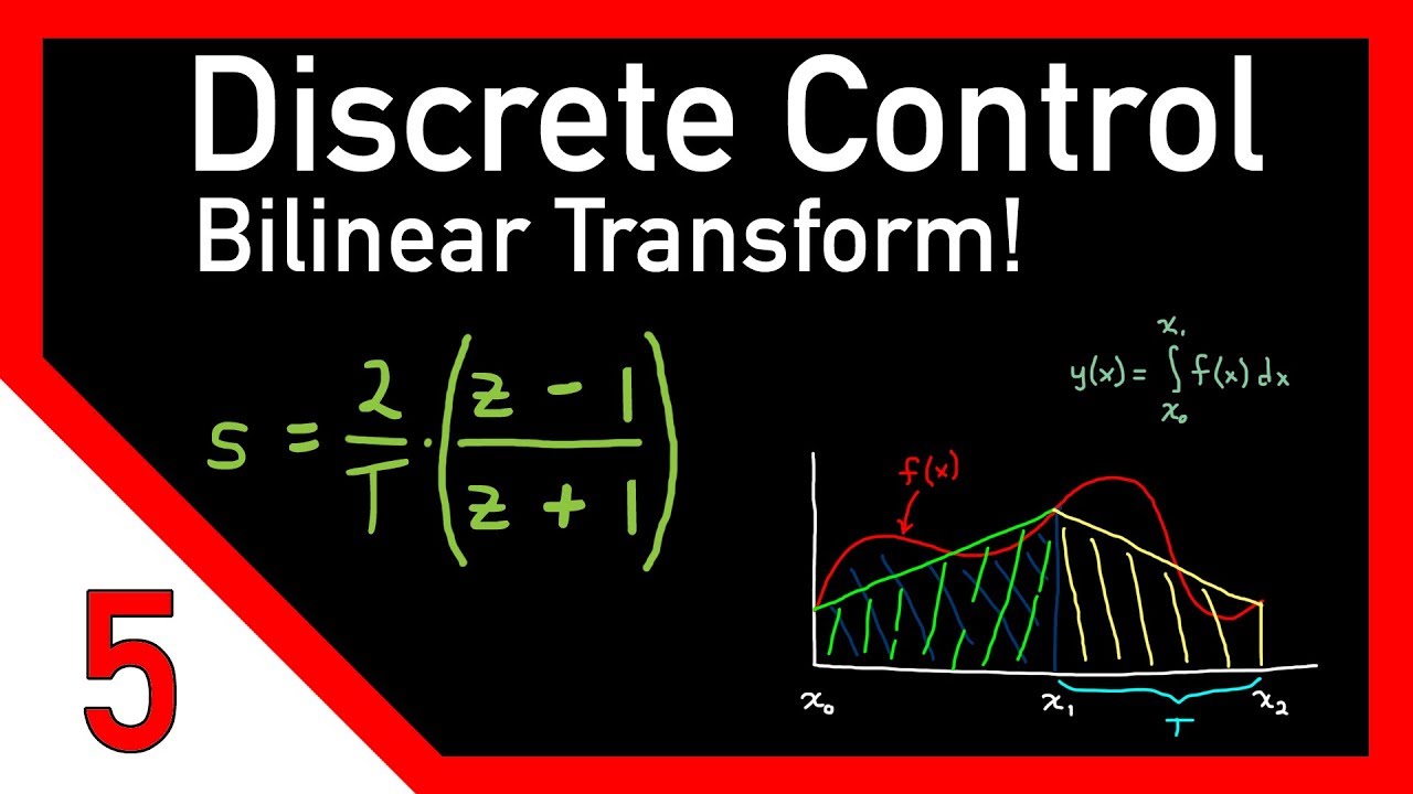
we're going to be using trapezoidal

integration let's start with a quick

refresher on trapezoidal integration

we're given a function f of X and we

want to find the following integral

basically we have some function this red

line and we want to calculate the blue

area under the curve between points x0

and x1 instead of solving the integral

directly we can approximate the area

with a trapezoid by drawing a straight

line between f of X 0 and f of X 1 this

works out that the original integral is

approximately equal to x1 minus x0 or

the width of the trapezoid times its

average height now if we add a second

point x2 and extend our red line

function out we can draw a second

trapezoid between X 1 and X 2 and the

approximated area for this next section

is drawn out in yellow but what is the

value of y between x0 and x2

remember why is the total area under the

curve so it's the old green area plus

the new yellow area the yellow area

again is the trapezoid width times its

average height and since y equals the

area into the curve the old green area

is actually the value of Y back at point

x1 and now we can generalize this to any

point X sub K with this equation its Y

sub K equals the width of each trapezoid

or Delta X times the average height or X

sub K minus 1 plus X sub K all divided

by 2 plus the old area Y sub K minus 1

all right with that out of the way let's

apply this integration to a system let's

say that our system is G of S which is

the transfer function with output Y of s

and input X of s and the whole thing is

equal to 1 over s we can rearrange the

equation to get s times y of s equals X

of s and then if we take the inverse

Laplace transform to get it back to the

time domain we're left with the

differential equation y dot of t equals

X of T now we can integrate both sides

to get Y of T equals the integral of X

of T DT and this is starting to look

really familiar you guessed it we're

going to use trapezoidal integration now

the first step is to change the variable

t to break it up into sample periods

capital T we haven't discretized in this

step it's still continuous because at

this point K doesn't have to be an

integer now we separate this one

integral into two integrals the first

one sums over the last sample period

capital T and the second one sums over

all of the sample periods not including

the last one you can see that the first

integral is the new area and the second

one is the old area just like we had in

trapezoidal integration all right at

this point we swap out the continuous

integrals with the trapezoidal

approximation x' so that the value of y

at KT is approximately equal to the area

of the new trapezoid plus the old area

this green equation is a bit hard to

understand so I'll write it in shorthand

notation Y sub K is approximately equal

to Y sub K minus 1 plus capital T over 2

times X sub K plus X sub K minus 1 at

this point it's worth noting that there

is no difference between the equation

for trapezoidal integration and this

equation that we just wrote the transfer

function 1 over s is just the transfer

function of an integral so it makes

sense that we got exactly an integration

equation ok from here we can rearrange

it into this difference equation and if

you haven't already made the mental leap

to where this is going then I think this

is gonna blow your mind it did for me

anyway

we take the z-transform of this

difference equation to get y of Z times

1 minus Z inverse equals T over 2 times

X of Z times 1 plus Z inverse and from

here we can rearrange to get the

transfer function y of Z over X of Z and

multiplied by Z over Z to put it in a

more pleasing form and we get T divided

by 2 times Z plus 1 divided by Z minus 1

recall our starting s domain transfer

function was 1 over s and so this is

equivalent to our Z domain transfer

function that we just solved for now all

we have to do is solve for s and we're

left with s is approximately equal to 2

divided by T times Z minus 1 divided by

Z plus 1 and I probably don't have to

tell you this but this is the bilinear

transform so the other way to think of

the bilinear transform equations is that

they are an approximation of

differential equations using trapezoidal

integration rather than continuous

integration I think that just makes a

ton of sense and is really cool alright

there's more we need to cover on this

but this video is getting really long so

let's take a break and we'll come back

with the second half of bilinear

transform in the next video and that one

will cover how it warps the S plane into

the Z plane how we can pre-warp an

analogue filter and I'll answer any

questions you might have on the topic

that pop up between now and the time I

put that video out so I'll see you next

video and thanks for watching and a huge

thank you to my patreon supporters for

making this video possible if you'd like

to support me and my efforts on youtube

you can from the patreon link in the

description below for any amount of

support you can download a digital copy

of my book in progress on control theory

now I'm still actively writing the book

so it's not complete but if you'd like a

copy of what I have so far but are

unable to support through patreon for

any reason at all just email me at

control system lectures at gmail.com and

I'll send you a copy for free

that way we can spread the knowledge and

help everyone on their quest to becoming

better control system engineers thanks

everyone