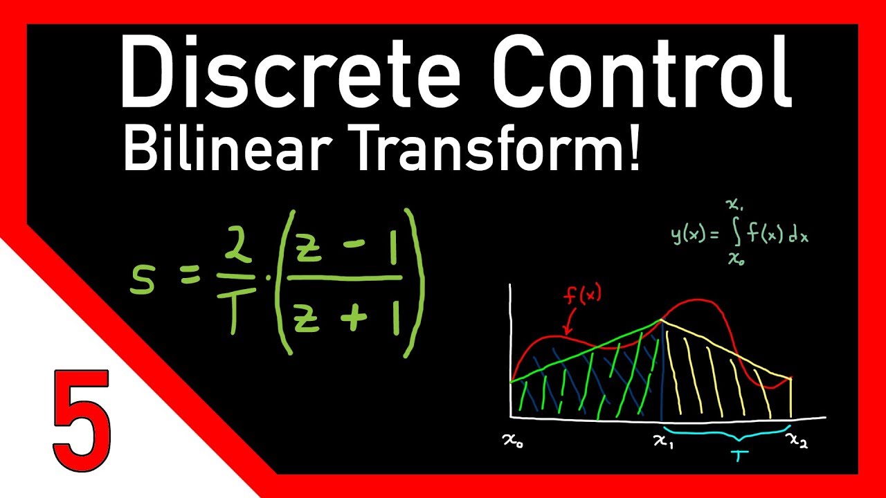
Discrete control #6: z-plane warping and the bilinear transform
Now Playing
Discrete control #6: z-plane warping and the bilinear transform
Transcript
630 segments
hey everyone welcome back to control
system lectures we're continuing our
journey through discrete control and in
this video we're going to expand our
understanding of the bilinear transform
and in doing so we'll learn about how
this transform warps the Z plane what
that means for us and what we can do
about it now this is going to be a
meandering journey but I think the
topics we'll cover will be necessary in
order to set up the proper context
around Z plane warping and this is like
a 25 minute video which is a long time I
know but to entice you to watch the
whole thing at the end there's going to
be this pretty sweet animation so
hopefully you stick around find out what
it is if you've missed any of the
previous videos on discrete control you
can find their links in the description
below let's get to it
there may come a time in your career
where you are asked to design a filter
that will be implemented on a digital
computer how do I go about doing this
you might ask a helpful friend and they
say it's easy just design a continuous
filter with the properties that you want
convert it to a discreet filter with the
bilinear transform and then tada you can
implement it on a digital computer which
you promptly try and find that the
performance is not what you were
expecting the frequency is all wrong why
is that well to answer this question we
first need to talk briefly about filters
you can think of a filter like a sieve
or a strainer that you'd use in cooking
its main purpose is to take a set of
items and remove specific unwanted items
from that set for example after you
finished boiling pasta you have a pot of
pasta and water you then passed the
combined pasta and water through a
strainer or a filter which will allow
the water to pass through and be
discarded so that you're left with only
the pasta
similarly filters can also be used on
signals like the voltage coming from a
sensor over time the voltage from the
sensor is changing and you can see the
frequencies that make up that time
domain signal by viewing it in the
frequency domain now you may not want to
keep the raw unfiltered signal because
it could be a mix of frequencies that
you want the pasta and frequencies that
you don't the water
so we can design a filter that removes
or stops the high-frequency signals from
getting through so that our system only
sees the low frequency sensor
information basically our system is only
getting the pasta in an ideal sense a
signal filter could be specified by
stating exactly which frequencies you
want to keep or pass through the filter
and which frequencies you want to stop
or reject with the filter these ideal
filters have names like low pass and
high pass and band reject or sometimes
called the notch filter and band pass
low pass filters keep frequencies below
the critical frequency and reject or
attenuate frequencies higher than it
high pass filters are the opposite they
keep the frequencies above the critical
frequency and reject those below it the
difference between these two filters in
our cooking example is whether you kept
or threw out the water for pasta you'd
keep the large low frequency noodles and
discard the higher frequency water but
for tea you would keep the water and a
few of the smaller high frequency tea
particles a notch filter is a low pass
and a high pass filter that don't
overlap such that there is a band of
frequencies in between the two that are
rejected and everything above and below
that band are kept you might set up a
notch filter if you're trying to remove
the humming noise and an audio system at
50 Hertz or 60 Hertz the one that's
generated by the powerline a bandpass is
the opposite of a notch filter such that
you only pass through a narrow band of
frequencies and everything above and
below is rejected for example our eye is
a bandpass filter for visible
frequencies in the e/m spectrum we can
only see those specific frequencies and
further still colored objects are
bandpass filters for that specific color
frequency if you shine broad spectrum
light onto a red apple only the red
frequency is reflected in the band that
our eyes can see and sometimes we only
want the metaphorical red frequencies to
get through our control system and in
that case we would design a bandpass
filter but these are ideal
representations of filters and we can't
expect to build a filter that perfectly
rejects or keeps fair
specific frequencies in our pasta
example sometimes a few noodles snake
their way past the strainer and there is
always some water leftover clinging to
the noodles in the pan so not a perfect
separation of the two in reality we're a
filter transitions from passing to
stopping is not a single point but
occurs over a band of frequencies
likewise you don't get perfect unaltered
frequencies in the passband region nor
do you always get perfect attenuation in
the stop band region how you design your
filter is based on the requirements for
the filtering that you are doing and
there are many variations of these types
of filters and their given names like
Butterworth and chebyshev and Bessel and
more and there's tons of them and
they'll probably be even more in the
future but the point I want you to take
away from this section is that almost
every filter will have these key
features in common and those features
are tied to specific frequencies so it's
important that our final digital filter
design maintains these critical
frequencies right where we want them it
does us no good to design a low-pass
analog filter only to have the
transition band move on us when we
convert it to a digital filter so with
that being said let's get back to our
original goal of designing a filter for
a digital computer like our helpful
friend suggested a popular way of
approaching this problem is to design an
analogue filter first get it just right
and then use the bilinear transform to
map it to the Z domain and hopefully
create a digital filter whose critical
frequencies have not been moved the
reason we would approach the design with
an analogue filter rather than directly
designing a digital filter is that we
have a large amount of continuous analog
Theory available to us that will give us
more tools to use during our design
let's see how this works in practice by
trying it out on a standard notch filter
at this point you've understood the
requirements your filter must meet and
you've toiled over the math and
simulations and you're happy with the
following analog filter design where
Omega naught is the critical frequency
that you want to attenuate which in our
case is 0.1 radians per second and Q is
the quality factor of the filter or a
value that corresponds to the steepness
and depth of the notch in this case
we're choosing Q equals 1
this will generate a magnitude response
curve that looks something like this
redlined now this isn't a video about
how to design an analogue filter that
would require its own standalone series
so I'm not going to go into detail about
how we chose this particular notch
filter for now just know that this is
one possible form of a notch filter that
we could have created to meet our
requirements and I'll show you in a bit
in MATLAB that this pink transfer
function does truly create a magnitude
plot that meets our requirements okay so
at this point we have a perfectly fine
analog filter but the catch as you know
is that we want to implement it on a
digital computer and say one running
with a sample time of two seconds which
means we need to map it to the Z domain
using the bilinear transform we did the
calculations by hand in the previous
video so in this one let's just go
straight to MATLAB first things first
let's define our Laplace variable s and
then set our sample time to two seconds
the critical frequency to 0.1 radians
per second and the quality factor to one
with our variables defined we can create
our S domain transfer function using the
equation for a standard notch filter and
no surprise we got the same result that
we did by hand now let's see the bode
plot to you check out the magnitude of
this filter across the frequency
spectrum and that's a good-looking notch
and if we zoom in a bit we can see that
the notch is located precisely at 0.1
radians per second just like we wanted
and we step one out of the way let's use
the bilinear transform or the Tustin
method to convert to the Z domain and we
get a discrete transfer function with a
sample time of two seconds so far so
good we can now plot the bode plots for
both the analog and digital filters on
top of each other and see how we did
that's that's pretty good the red
digital filter lies pretty much on top
of the blue analog filter we did some
fine work here
and all that's left to do is write some
code for this filter and put it on our
digital computer oh wait a second I I'm
just realizing that I got our original
requirement wrong it looked like Omega
naught was written as 0.1 radians per
second but really it was supposed to
read 0.7 Radian
per second okay that's no problem we'll
just update the omega-not variable 20.7
rerun our analog transfer function and
discrete-time transfer function now this
is probably still okay but let's just
check the bode plot once again to be
absolutely sure and they're different
and if we zoom in we can see that the
analog notch is at 0.7 like we want but
the digital notch is much lower at 0.6
one radians per second what happened all
we did was increase the critical
frequency
well this shift in frequency comes down
to how the Z plane is warped by the
bilinear transform differently than e to
the St which is the true definition of Z
so it should be clear that you can't
just blindly apply the bilinear
transform to any function with any
sample time and get a good match in the
Z domain so what's going on here to
answer this we must first talk about how
Z equals e to the St maps from the S
plane to the Z plane I'll just set up a
blank s plane and blank Z plane and
let's try to convert a few points for a
sample time of two seconds we'll start
with the origin s equals zero plus zero
J this gives us Z equals e to the 0 or 1
so the origin in the S plane maps to the
point 1 0 in the Z plane let's try s
equals minus 1 plus 0 J and this maps to
zero point 1 3 5 3 in the Z plane this
is inside the unit circle and fairly
close to the origin if we head up the
imaginary access to s equals 0 plus J we
see that this maps to negative zero
point four two plus zero point 9 1 j
which lies on the unit circle in the z
plane and finally let's try a point at s
equals minus 100 which is practically
negative infinity for this system and it
maps to one point three eight times ten
to the minus 87 basically zero so points
near negative real infinity mapped to
the origin in the Z plane
doing math is fine you know it's fine
but I think it helps to be able to
visualize the mapping here's what it's
doing we start with the Cartesian grid
in the s plane the e to the real part of
s scrunches the left half plane inward
to where the entire left half plane
exists between the real values 0 and 1
and the right half plane extend out past
1 to infinity the e to the imaginary
part rotates this scrunched grid around
the origin and it just keeps rotating it
more and more as Omega increases towards
infinity in this way the J Omega line in
the S plane maps to the unit circle in
the Z plane now to help with this
visualization let's look at something
much more precise than my drawings I
wrote a little program that maps a
location in the S plane on the left to
the Z plane on the right using the
transformation Z equals e to the st and
in this case T is set to 2 seconds
you'll note that the left half plane is
gray and this maps entirely into the
grey unit circle in the Z plane the
right half plane the white part is
outside of the unit circle the origin of
the S plane the red dot is mapped to the
point 1 0 the black dot now if I move
that red dot to about minus 1 0 you can
see the black dot moves inward towards
the origin and if we keep going more
negative in the S plane it pretty much
Maps right onto the origin of the z
plane and if we start heading up the J
Omega axis the black dot follows the
perimeter of the unit circle that's
because the J Omega axis maps to the
unit circle in the Z plane now here's
the interesting part if we start at a
fairly negative J Omega value and just
start increasing it you'll notice the
black dot rotates around the origin
again and again this is the effect the
imaginary part has on the mapping it
just rotates the mapping around the
origin while the real part dictates how
far you are from the origin now keep
that in mind as we contrast this
behavior with the bilinear transform
we'll start by drawing out a blank s
plane and Z plane again and then convert
the same four points that we did with e
to the S T but this time using the
bilinear transform we'll start with the
origin in the S plane which maps to the
point plus 1 in the Z plane the same as
we got before but this time the point s
equals minus 1 maps exactly to the
origin in the Z plane and the point s
equals 0 plus J maps to J in the Z plane
now that's still on the unit circle I
mean the J Omega lines still maps to the
unit circle using the bilinear transform
but the resulting location around the
circle has changed finally our point at
basically negative infinity maps to
about minus 1 in the Z plane the math is
the math but just like we did before
let's attempt to visualize this mapping
and see if we can use that visualization
to understand how these two transforms
project the S plane onto the Z plane
differently again we start with the
Cartesian grid in the S plane but
instead of scrunching it in from the
negative real line we're going to pinch
it in at three different locations we're
gonna bend the J Omega axis down from
the top and up from the bottom so that
the tips of the line at positive and
negative infinity meet at the point
minus one similarly we're going to pinch
the negative real line so that it's
infinity also meets at minus 1 with this
mapping there are no rotations just a
pinching of the positive and negative
imaginary infinities and negative real
infinity so that they all meet at minus
1 again the pinching is done such that
the J Omega line wraps around of the
unit circle now let's see what this
looks like with a bit more precision
this is the same idea as before but now
we're going to map from the S plane to
the Z plane with the bilinear transform
still with a sample time of 2 seconds
just like with E to the s T the bilinear
transform maps the entire left
half-plane to inside of the unit circle
but now look at the way that this grid
in the Z plane is shaped compared to the
one that we saw with E to the s T the
grid gets more dense towards -1 rather
than the origin and if you follow the
real or imaginary lines in the S plane
they all curve towards this minus 1
point in the Z plane the origin in the S
plane mapped to the point 1 0 as we
expect and as we move along the negative
real line we can watch the black dot
also move along the negative real line
closer and closer to minus 1 but never
quite reaching it and if we move up and
down the J Omega line you can see the
black dot travel along the unit circle
towards minus 1 as well so all
infinities in this left hemisphere in
the S plane mapped to minus 1 in the Z
plane a bit different than e to the St
for sure ok what does this difference in
warping have to do with the frequency
well let's take the bilinear transform
and recognize that s is defined as Sigma
plus J Omega Sigma is the exponential
term which doesn't impact frequency so
we can just look at J Omega for
frequency information we can plug J
Omega into the bilinear transform for s
and we get this equation here I wrote
Omega sub a for analog frequency because
this was the true s domain location
which defined the analog frequency that
we wanted this was our starting point
however to find out what this new
frequency is that we just created we can
convert back to the S plane using the
definition of Z or e to the S T for this
s I'll replace it with Omega sub D for
the discrete frequency that resulted
from the bilinear transform now we can
just solve for Omega D as a function of
Omega a and you can tell from this
equation that Omega D does not equal
Omega a we've moved the frequency by
using the bilinear transform we can
simplify this equation but for now let's
try a few points with this unsimplified
equation and see how the frequencies
move but before we do that let's
recognize that for a sample time of 2
seconds or a sample frequency of 1/2
Hertz the Nyquist frequency is 1/4 Hertz
or half the sample frequency this puts
the Nyquist frequency at PI over 2
radians per second and we're going to
use this shortly for our first point
let's look at an analog frequency of 0.1
radians per second this is about 6% of
the Nyquist frequency which is
relatively slow let's plug this into our
equation and rather than solve it by
hand let's just quickly solve it in
MATLAB first I'll define the Omega a
variable type out the equation for Omega
D and we get a discrete frequency of
zero point zero nine nine seven radians
per second you'll notice that this is
very close to our starting analog
frequency and it's what we saw when we
plotted the discrete and analog notch
filters on top of each other when the
critical frequency was zero point one
radians per second now let's try an
analogue frequency of zero point seven
radians per second this is a relatively
fast frequency or about 45% of the
Nyquist frequency again we set up our
equation to solve for Omega D and then
we go back to MATLAB change our Omega a
variable and solve for Omega D the
discrete frequency is not zero point
seven radians per second but about zero
point six one which again if you recall
was the difference we saw between our
two notch filters when the critical
frequency was 0.7 radians per second
interesting so at this point you might
be asking what happens if we design a
filter above the Nyquist frequency well
let's try it with an analog frequency of
2.5 radians per second well zip through
the math real quick you can double-check
this on your own but we find that it's
about one point one nine radians per
second which is really different than
our goal
it was mapped to just below the Nyquist
frequency in fact it doesn't matter how
high the analog frequency is when you
map that system using the bilinear
transform it always maps it to just less
than the Nyquist frequency that's the
result of the mapping not rotating
around the origin but rather pinching it
down to minus 1 that minus 1 point is
the Nyquist frequency in the Z plane ok
enough of that the question is what can
we do about this
well remember I said that this equation
can be simplified the math is pretty
straight forward to do the
simplification but it's a bit much to
write out here instead I direct you to
follow along with the Wikipedia page
where they do a pretty good job of
deriving the simplified equation and
it's this equation here where Omega D is
this arctan function of Omega a alright
we are in the homestretch now I'll
rewrite the frequency warping equation
here and if we plot this equation we
find something very telling as we
increase Omega a Omega D continues to
increase as well but asymptotically to
PI over T which is the Nyquist frequency
in our case it's PI over 2 since our
sample time is 2 seconds and what you'll
notice is that this equation has nearly
a one-to-one linear relationship with
Omega a and Omega D at low frequencies
compared to the Nyquist frequency and as
we increase Omega a Omega D differs from
it more and more just like we saw with
our design so ask the question again
what can we do about this well we can
pre-warp Omega a essentially this means
that we are artificially moving our
design frequency before mapping it with
the bilinear transform so that after the
mapping the critical frequency is in the
correct spot to do this we apply the
tangent equation to Omega a first
luckily there is a way to do this pre
warping at the exact same time that we
do the bilinear transform with a
modified version of the transform
instead of having a multiplier of 2 over
T we multiply Z minus 1 over Z plus 1
with Omega naught divided by the tangent
of Omega naught times T over 2
and you know we could do this mapping by
hand but again we could just do it in
MATLAB as well once again we'll set up
our variables and define our S domain
notch filter at zero point seven radians
per second
then we can convert it to the Z domain
with the bilinear transform but this
time we'll apply a pre warping at zero
point seven radians per second during
the conversion remember when we did this
without the pre warping our discrete
knotch filter came back at zero point
six one radians per second so let's see
how this one does and it's perfect look
at this if we zoom in we can see that
with the pre warping we were able to
create a notch filter with the desired
critical frequency okay that's pretty
much what I wanted to cover in this
video just that we can use the bilinear
transform to convert analog filters into
discrete filters but we have to
understand how frequencies are warped
during this process and account for them
during the conversion so thanks for
watching and following along with this
extremely long video but before I leave
you I promised that we would end with a
pretty sweet animation well I think it's
sweet anyway once again I present the Z
plane and it's unit circle I'm going to
use this to show you exactly what is
happening when we apply a pre-warp at a
specific frequency I'm plotting four
poles here the two on the far right are
the two notch filter poles for the
critical frequency of 0.1 radians per
second and the two on the left are the
notch filter poles for the critical
frequency of 0.7 radians per second
these are the true locations of the
poles when converted using Z equals e to
the St the grid pattern you might
recognize as the mapping that occurs
when using e to the S T now I'll add on
top of this the exact same for poles but
this time mapped using the bilinear
transform notice the two on the right
overlay nicely this agrees with what we
saw before which was that relatively low
frequencies compared to the Nyquist
frequency don't get shifted by very much
however look at the two poles for the
zero point seven radians per second
critical frequency not close and also
exactly what we saw before now watch as
I apply a
pre-warp at a larger and larger critical
frequency the whole red grid starts to
move and stretch and moving the poles
along with it and if I stop exactly at
zero point seven radians per second you
can see that all four poles for the zero
point seven Radian per second notch
filter line up with each other
now in doing so the four zero point one
Radian per second poles no longer line
up but that's the penalty we have to pay
with the bilinear transform we have to
choose the frequencies that matter most
to us but all in all the bilinear
transform is pretty awesome okay that is
the end of this video
finally a huge thank you to my patreon
supporters for making this video
possible if you would like to support me
in my efforts on youtube you can from
the patreon link in the description
below for any amount of support you can
download a digital copy of my book and
progress on control theory now I'm still
actively writing the book so it's not
complete but if you would like a copy of
what I have so far but are unable to
support through patreon for any reason
just email me at control system lectures
at gmail.com and I will send you a copy
for free
that way we can spread the knowledge and
help everyone on their quest to becoming
better control system engineers thanks
everyone
Interactive Summary
Ask follow-up questions or revisit key timestamps.
Este vídeo explora o funcionamento da Transformada Bilinear na conversão de filtros analógicos para filtros digitais. O autor demonstra que essa transformação causa um fenômeno conhecido como "empenamento" (warping) das frequências, onde as frequências críticas do filtro original não correspondem exatamente às do filtro digital resultante. Após explicar a diferença entre o mapeamento do plano-S para o plano-Z usando a função exponencial e a transformada bilinear, o vídeo apresenta a técnica de "pré-empenamento" (pre-warping) como uma solução para alinhar corretamente as frequências críticas desejadas.
Suggested questions
2 ready-made promptsRecently Distilled
Videos recently processed by our community