Welcome back. So, we are just kicking

off this boot camp on optimization and

so I thought I would give a more

in-depth discussion on some of the many

many applications of optimization in the

modern world. Now, this is kind of too

big of a topic for one lecture or even a

lecture series. It's like asking you

know what are the applications of

calculus or statistics or linear

algebra. Optimization is everywhere. It

is ubiquitous in almost every modern

industrial technology. But I wanted to

highlight some of the ones that I'm

going to focus on in particular in this

lecture series and some of the

applications that I'm particularly

motivated by and think are changing the

fastest and have the biggest

opportunities in the future. Okay. So uh

big big categories are going to be

things like machine learning uh control

theory and inverse uh inverse problems

and inverse design. Those are kind of

the three big areas I'm going to talk

about. things I'm going to gloss over

and I'm going to go into, you know,

specific lectures I might bring these up

are things like finance, supply chain

optimization, scheduling, you know, how

do you make an airline uh have the most

on-time departures, things like that.

Those are all really important

applications of optimization. Making

sure that you have minimized network

downtime in, you know, internet traffic

and things like that. uh optimizing the

LA traffic network. You know, those are

all really, really important

optimization problems. I'm going to

focus on machine learning, on control

theory, and on inverse problems and

design primarily as kind of my

motivating examples, my lighouses. But

whatever you're interested in, I can

almost guarantee optimization has some

part in it. Okay, so let's start. Um I'm

going to zoom in to begin with just with

machine learning. So let's get into to

machine learning.

um pretty much any machine learning

model that you have ever used or that

you have ever trained used optimization

under the hood to train that model. So

generative models uh chatgpt you know

dolly to uh all the way to really really

simple models that you would use are um

all based on optimization. So not all of

machine learning is neural networks but

I think this is a nice illustrative uh

picture that can help us think about how

optimization applies to machine

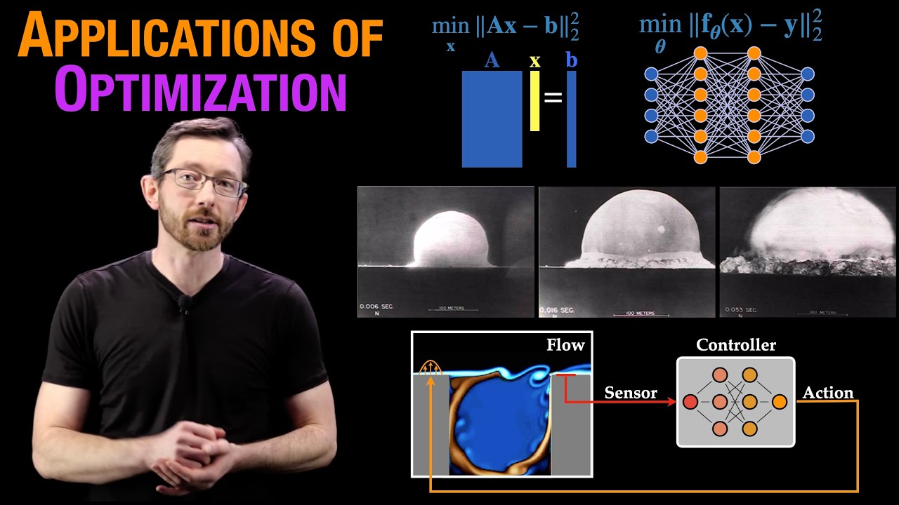
learning. Generally speaking a machine

learning model is trying to build some

model between inputs x and outputs y and

there are some parameters theta you get

to tune to to tune that function uh to

capture that input output relationship.

So this might be you know pictures and

these might be labels of the pictures or

something like that. This might be a

low-res image. This might be a high

resolution image. Things like that. And

you know the parameters theta in this

case would be the parameters of the

neural network that I get to tune and

optimize over to get the best model

approximation possible. Um the weights,

you know, of all of my uh connections in

my neural network. This is not an

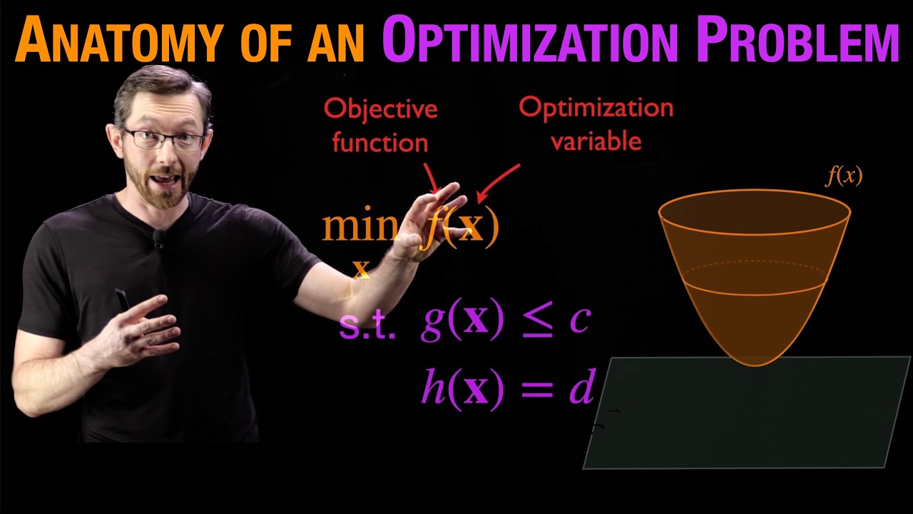
optimization problem. This is my

objective of what I want my machine

learning model to do. I want to take

input data X and predict output data Y

with this function f. I can turn it into

an optimization problem in the following

way. So now what I'm going to really try

to do is I'm going to try to minimize

the mismatch between my model and actual

data by minimizing over these free

parameters data. Now I've turned my

machine learning training problem into

an optimization problem. And again under

the hood all the time anytime you train

a machine learning model you are doing

some kind of an optimization probably

something like stochastic gradient

ascent using atom in you know pietorch

or jax or tensorflow. Okay but it is an

optimization

problem. Uh the kind of more classic

historical you know um precursor of

machine learning is le squares

regression. So, you know, similarly, I

might have some model that fits my data

where I'm trying to to solve for this

unknown vector of coefficients X in some

kind of a big linear regression model

and I'm trying to find that X that

minimizes the sum of the square of the

errors over my data. So, this is the

basis of principal components analysis,

singular value decomposition,

dimensionality reduction, factor

analysis, most of highdimensional

statistics. And we can do things like

take highdimensional images either of

you know physical systems like a fluid

flow or a person's face and decompose

them into a minimal number of kind of

basis features. You could find these

optimal basis features in some kind of a

lease squares regression optimization

procedure. Okay. Again hugely hugely uh

important in image classification

reduced order modeling all across the

board in science and technology. We use

le squares everywhere. Okay. This is an

optimization

problem. Okay, back to to kind of more

modern machine learning optimizations.

If I have a neural network, um I have a

loss function where I'm trying to fit uh

I'm trying to to build a model that fits

my data. I've changed my notation a

little bit here. I could also add

physics into this neural network

problem. So that's something I'm very

concerned about as an engineer is when I

use machine learning on engineering

systems, I want to bake in physics that

I know. You can again do that. You can

again do that in your optimization

procedure by adding terms to your loss

function. This is your loss function,

your objective function you're you're

optimizing over. You can add terms that

says that your um you know your system

has to be physical. So if you know that

there's some partial differential

equation that these variables have to

adhere to, you can add that in the loss

function. And with modern machine

learning training, you can evaluate this

function. You can compute its gradients.

you can optimize the weights of your

neural network um to also minimize this

loss function as well. Okay, so again um

really really important in the modern

era optimization is what allows you to

encode physics into your machine

learning

algorithms. There are other ways. So

that was by adding a term in the loss

function and then using classic machine

learning. There are other approaches

where you can actually do constrained

optimization. You can set up constraint

equations that have to be satisfied for

your system to be physical. So this is a

really cool example. I'm going to have a

whole lecture on this later. Um this was

inspired by Jean Kristoff Loazo. Um

trying to model fluid flows using really

kind of simple generalized linear

machine learning models. So he's trying

to get differential equations that

describe this behavior, this complex

behavior with a reduced order model. But

what JC realized is that instead of just

including this model error, you want

your machine learning model to have a

good fit. This is just your fit. Le

squares fit. He also realized that for

this to be physical, if you actually

write down the equations of motion,

Navier Stokes equations for fluids,

there are certain constraint equations

that you can derive on the coefficients

of this le squares model. So, so we're

trying to do le squares optimization to

find these coefficients C. But JC

pointed out that these coefficients have

some symmetries that you can encode in

constraint equations. So now he writes

this as a

minimization subject to some

constraints. In this case, this is the

lrange multiplier form plus some lrange

multiplier zrpose times these

constraints. And that is solvable with

this KKT constrained le squares

optimization. So again if you have this

machine learning problem you're trying

to build a reduced order model for a

very very complicated process and you

have some prior knowledge some

constraints from physics you can add

that as a constrained uh optimization

problem. Okay so again we'll have a

whole lecture on this but um adding

physics into machine learning is very

often done by either adding a loss a

term in the loss function or adding

constraint

equations. Now those constraint

equations uh very often come up as

either subspaces or submanifold

constraints on the feasible set uh of my

variables x. So what I mean by physics

and putting physics into machine

learning usually means symmetry. So we

are used to seeing this in convolutional

neural networks. We know that natural

images have translational symmetry. Um,

physical systems often have rotational

symmetries, scale symmetries, and those

symmetries are uh determined by symmetry

groups. And those symmetry groups

determine essentially manifolds that

constrain the feasible set of X's uh

that my my machine learning model can be

optimized over. And so you can again

either have your minimum error uh term

in your loss function. You can add terms

that project onto these manifolds or you

can actually do a constrained

optimization where you are minimizing

the sum of the squares of the error

subject to your variables being you know

on this manifold or on this subspace. So

again um that's kind of this dual notion

that I can either add penalty terms to

my loss function or I can add hard

constraints um in my optimization

problem. But most of physics is encoded

in symmetries and invariances like

rotational symmetry and translational

symmetry and those are possible to bake

into your machine learning algorithm

with uh various optimization techniques

that we're going to talk about. Good. Um

okay so machine learning is a huge huge

category I care about I think about all

the time in the context of optimization.

Optimization is the engine that powers

machine learning. data is the fuel. Um,

now we're going to zoom into control

theory. Okay, so control theory is

another huge category that motivates me

to study optimization

theory. So a control problem where you

have some dynamical system and you have

you can sense it, you can actuate it.

Maybe there's disturbances and there's

some objective or cost function that

you're trying to optimize over. You're

trying to design a controller that

manages all of this that you know uh

determines the actuators based on the

sensors to minimize a cost function

given external disturbances. For

example, the cruise controller in your

car or trying to stabilize an inverted

pendulum or a rocket that's rellanding

back on Earth. Now, what makes this a

really really cool optimization problem?

Almost all control theory can be posed

as an optimization problem subject to

the constraints of the dynamics of your

system. So in the case of a rocket, it's

like an inverted pendulum. Um the cruise

controller on your car, your car has

momentum, you know, inertia, it has

physics that determine the rules, the

dynamics that that system has to

satisfy. So control theory can be

thought of as a constrained optimization

problem. You're trying to find the

control input u maybe the minimum

control uh to achieve a desired

objective subject to the constraints of

the

dynamics. Reinforcement learning is like

control theory on steroids where

nowadays we are using machine learning

to either learn the controller directly

or to learn surrogate models of the

dynamics so that you can speed up uh the

the reinforcement learning training. But

again, both of these cases of kind of

classical control and reinforcement

learning are under the hood posed as

optimization problems. So all of the

robust control toolbox in Python in mat

lab is basically wrapped around forrren

codes that were written approximately

the year I was born that solve linear

matrix inequality optimization problems.

Okay, so all of robust and you know

optimization and control is based on

these optimization toolboxes.

And this is changing how we do robotics.

It's changing how we control fluid

flows. Lots and lots of systems of

control systems are advancing because

our optimization techniques are getting

much better because we can uh build

again good surrogate models for the

forward model or for the controller with

machine learning and we have powerful

optimization tools and more data to

build better controllers. So control

theory is going to be a huge area again

a whole chapter and a whole unit in this

uh this series is going to be on

optimization for control theory. So

optimization for machine learning

optimization for control theory and kind

of the third big piece I think about all

the time are inverse problems. So

inverse problems um and inverse design

problems. you know, how do I if I have

some specifications, how do I back out

the aerodynamic shape and the materials

and the manufacturing process that will,

you know, that will satisfy those those

design criteria? So, in general, inverse

problems are related to optimization um

but they're slightly different. So, an

inverse problem, I would have a forward

model f ofx and I would have some

observed data y. I would have some

observation and I'm trying to back out

what is the X that is most consistent

with that forward model and that

observation Y. You could think of this

as a Beijian inverse problem. Very often

we do inverse problems in in statistics

with B theorem. Uh this is not an

optimization problem but you can write

this as an optimization problem by

trying to find the argument. Again, I

want to find the X that minimizes the

mismatch between my model and my

observations. That's how to turn an

inverse problem into an optimization

problem. Okay, inverse problems are

massive. I'm going to give you just the

barest hint of some of the applications.

And again, I'm going to have a whole

chapter, a whole unit on inverse

problems and optimization

later. So, I mean, there's so many it's

not even uh really fair to have this

only have a couple of minutes. This is

going to I'm going to have a whole

overview video just for inverse problems

and we're going to have a whole, you

know, chapter and unit on this. Um, one

of my favorite examples of this is this

really cool historical example. So, this

is a series of four still images from

the Trinity tests um of the first atomic

bomb. And these were published in a

popular science magazine. And the famous

British physicist GI Taylor took these

four images. You'll notice here it has,

you know, what time uh these were

exposed at. And there's also a little

distance bar here. It says, you know,

how large whatever 100 meters is. So, GI

Taylor took kind of the distance, the

radius of this uh mushroom cloud over

time and used dimensional analysis and

physics to back out the unknown

quantity, the yield of this bomb just

from these four images. That's a classic

example of an inverse problem. I think

it's a really cool example of

dimensional analysis, too. But that's

kind of what we mean. We have observed

data. How would you back out the yield

just from this very limited information?

that's an inverse problem. Um, pretty

much all of medical imaging is an

inverse problem. So, um, MRIs and CT

scans are, you know, there are these 2D

imaging slices that you take of a

person's body, usually by shining light

through an entire section of of flesh

and bones and integrating over that

line. And then you have to do some kind

of an inverse transform, usually like an

inverse radon transform to get these

nice clean tomographic images that

doctors can use to detect cancers or,

you know, traumatic brain injuries. This

has revolutionized

uh the medical profession, medical

imaging. This is all a massive massive

inverse problem. The data you have is

not clean 3D images. It's weird line

scans through tissue and you have to

back out the 3D images.

More recently, one of the most kind of

exciting examples of this uh we are now

able to image black holes using

earthbased satellites or you know

satellites in earth's orbit. So a

distributed set of sensors at different

radio um you know kind of

electromagnetic frequencies are able to

stitch together that information and

piece together these beautiful pictures

of uh of black holes. And again, that's

a huge inverse problem. We are not

measuring this picture. We're measuring

all kinds of weird direct indirect um

sorry, we're measuring indirect uh

pieces of evidence and we have to invert

that through some model to get the thing

we want, which is a picture of a black

hole. So all of these are inverse

problems. Now, inverse problems uh are

probably most commonly seen in the

imaging sciences. So super resolution is

a great example. If I have a blurry

image and I want to find what is the

most likely highresolution image that

gave that that blurry image, that's

called super resolution. That's an

inverse problem. It's ill-posed because

there are infinitely many high-res

images that could have given this. And

so you have to regularize the problem

with optimization to make this a

well-posed optimization problem. Now

inverse problems are, you know, if you

think about it, actually control theory

and machine learning are both kind of

inverse problems. I'm trying to invert

the model parameters theta or I'm trying

to invert the control signal you know u.

And so inverse problems is almost like a

superset of all of those. But solving

inverse problems is also improving a lot

with machine learning. So better forward

models that you learn with machine

learning can improve this inverse uh

problem

procedure. Okay. So image uh super

resolution. Another really cool example

is dnoising or debluring. So if I have

this movie of a physical flow past a

cylinder, an inverse problem would be

could I separate this out into two

movies? One that has no noise and one

that just has the noise. This seems too

good to be true, but modern optimization

actually makes this possible. This is

the actual results of an algorithm run

by Isabelle Shur. Um, and it's

essentially this is the optimization

problem you're trying to solve. I'll

talk more about this. You know, L um is

low rank, so we're trying to minimize

the rank of L. S is sparse, so we're

trying to minimize the zero norm of S.

This is non-convex, so you actually have

to convexify it. And then you can solve

this optimization problem and get this

kind of amazing uh decomposition. So

this is an inverse problem. This is the

power of inverse problems and modern

optimization. It's all based on

optimization.

uh model discovery and physics discovery

is an ill-posed inverse problem. So I

have observed data and I want to learn

what is the best differential equation

that best describes this and has as few

terms as possible that's as

interpretable to a human as possible.

Again you can write this as an

optimization problem. You build a

library. You do le squares regression

with some regularization terms to make

your optimization well posed. Now you

have an optimization problem. model

discovery is typically posed as an

optimization problem. This is an inverse

problem. What model best describes my

observed time series data? And here's

kind of a cool movie actually just

seeing this optimization working. So

here we're trying to find a simple model

and a good coordinate system uh for

model discovery. And you can actually

see this optimization happening in real

time. Um this is probably performed in

like PyTorch or TensorFlow a modern

machine learning optimization uh

framework and you can see this kind of

optimization happening in real

time. Other really really big categories

of inverse problems um some inverse

problems involve really complicated

physics. So the forward model F might be

a huge simulation of you know vibrations

and elastic dynamics in the earth. If

you're trying to do something like

seismic inversion, maybe I have

measurements, uh, you know, seismographs

at different locations on the earth's

surface and I want to pinpoint where an

earthquake occurred and how big it was.

That is a a constrained inverse problem

constrained by the partial differential

equation of, you know, the elastic

dynamics of Earth and its interior. Very

very hard problem. Very important

inverse problem. And again, an inverse

problem that's being advanced heavily

with with advanced optimization

techniques and improved machine learning

techniques. And all of this culminates

into better industrial design, better

industrial processes. You know, those

are also kind of inverse design

processes. um you know if I have some

specifications I want this engine to run

20% hotter or I want this alloy to be

20% stronger or have 20% you know higher

melting point or I want this airplane to

be 20% more fuel efficient than its

predecessors those are all really really

hard opation problems but typically you

use some kind of inverse design you have

some forward model either you actually

build them and test them and iterate

over your design parameters or you

simulate them in a computer. Um, but

that at the end of the day is kind of an

inverse problem that is heavily rooted

in optimization. So things like

aerodynamic shape optimization,

composite materials or alloys, engine

performance, all of these are inverse

design uh,

optimizations. And again, I've been

saying that machine learning is helping

us do better inverse design and better,

you know, solve these inverse problems

better. A lot of this culminates in

what's known as the digital twin where

you have some device you're trying to

optimize or control um you know or or

monitor like an aircraft. You would want

to have a digital surrogate model that's

much much cheaper to optimize over much

cheaper forward model and that's going

to allow you to use much more powerful

iterative uh solution techniques to

solve that inverse problem. If you have

a cheap digital surrogate model, you can

do a lot more iterations of that forward

model to solve this inverse problem of

for example improving lift or decreasing

drag or making you know the structure

stronger or you know more durable things

like

that. And so one of the ways I see this

I'm going to have a whole uh series on

digital twins and and and this later is

in the modern world we actually have

lots of different fidelities of data. If

I'm trying to design something like an

aircraft or a race car or really

anything, I'm going to have different

fidelities of data both simulations and

experiments. And what I want to do is I

want to synthesize that into a better

forward model. Okay, that is called a

surrogate model sometimes. Sometimes

it's called a digital twin. Sometimes

it's just called a reduced order model.

This itself requires optimization to

build this model to synthesize this data

into the best fit model. That's a

machine learning problem. And that's an

optimization problem. But then I would

want to use this cheap inexpensive

surrogate model to do my inverse design

optimization over to to to test in

simulation what would happen if I

changed the geometry or I changed the

material or I made this structure longer

or shorter. Very expensive to do it here

very inexpensive to do it here in the

digital twin. So that's another area

where optimization uh is really really

changing how we do engineering is both

in building these surrogate models with

machine learning based optimizations and

then doing actual optimization of real

physical devices by optimizing over that

surrogate model. Okay. So um and if you

are clever sometimes your model will

have to go get more data. If you're

optimizing into a region you've never

seen before you might need more data. So

that's active learning.

which is an optimization problem. Okay,

so that was the mile high view of some

of my favorite applications of

optimization. We're going to dig into

each of these later. Have kind of a

whole chapter and a whole unit on

optimization for machine learning,

optimization for control and

optimization for inverse problems uh

more generally. All of that's coming up.

But that for me is kind of the

lighthouse set of motivating examples

when I think of optimization. We're

going to get pretty into the weeds in

math, convexity, non-convexity, feasible

sets, polytopes. You know, we're going

to do a lot of math so that we can solve

and understand the structure of these

optimization problems. But this is why

we do it. Okay? So that we can solve

these really important problems. And

these are all outstanding problems.

There is room to be improved in every

single aspect of control theory, of

machine learning, and of inverse

problems. So these are going to be

relevant for decades to come. These

techniques are going to be valuable. If

you know how to use optimization in any

one of these, you're going to be able to

help, you know, do really, really cool

things in the future. All right. Thank

you.