Welcome back. So today I'm excited to

tell you about the anatomy of an

optimization problem. Literally what

makes an optimization problem? How does

it work? What are all the pieces? Before

I do that, I want to just remind you

that optimization is one of the most

ubiquitous topics in all of applied

math. It is used everywhere in our

modern industrial world. Anytime you

have ever used or trained a neural

network or any machine learning

algorithm, you're using optimization to

minimize the loss function uh of that

that machine learning model fit. Same

thing is true for the more classic le

squares uh regression we use in data

fitting all the time and in statistics.

This is true basically all of control

theory is a constrained optimization

problem. Uh and most of our industrial

technologies involve optimization almost

at every stage. Uh designing engines and

aerodynamics and materials and you know

airline logistics and scheduling all of

this is optimization. So optimization

really is everywhere. Um I'll have a

whole lecture on on applications of

optimization later. But today I want to

give you uh a really highlevel quick

overview of what is the anatomy of an

optimization problem. What are the

pieces? How do they work? What are they

called? And what are some of the

textures that distinguish some

optimization problems from other

optimization problems? So, let's get

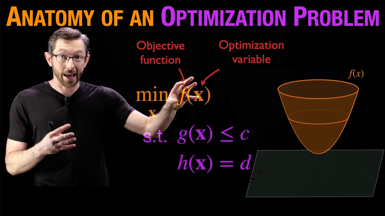
started. An optimization problem all

starts with this humble objective

function. So, f is our objective

function. In this case, we're trying to

minimize f over some variables x. X are

the variables that we get to optimize

over. Okay. So, um, you know, maybe I'm

trying to minimize the cost of something

or I'm trying to minimize the error of

my machine learning fit. That would be a

really good example of an f ofx. This

could be the sum of the squares of the

errors of my my machine learning model

averaged over all of my training data.

Okay. And so this objective function

usually I'm going to write f as a

scaler. I'm going to say that there is

one thing I'm trying to optimize. It is

you know again maybe that that sum of

the squares of the errors and my

optimization variable the variable I get

to tweak to minimize this f that might

be very highdimensional. X might have

you know one component two component or

two million components in the case of a

neural network. I might get to tweak all

of the weights of all of the layers um

and all of the connections that might be

my variables x. Okay so that is my

objective function. Now, of course,

sometimes I want to maximize f ofx.

Maybe I want to maximize profit or

maximize productivity and that's also

totally valid. But this is kind of the

standard form we're going to be writing

things you in most of the time is as a

minimization problem. Maximization is

you know basically just the opposite. So

everything I say for minimization is

also going to be true for maximization

problems. Um and our objective function

f here in two dimensions. You can see,

you know, there's lots of of examples of

f ofxs that we might want to optimize

over, but here our f ofx is a nice

simple kind of two-dimensional bowl over

a two-dimensional state variable

x. The next ingredient in an

optimization problem is a set of

constraint equations. Now, sometimes

I'll have an unconstrained optimization

where x can take any value I like as

long as it is, you know, minimizing f.

Other times I'm going to have

constraints on what values X can take.

There might be constraints like X has to

be non- negative. I can only have

positive X's or maybe X's can't be too

big. I I need, you know, X to be less

than some value. And there might be more

complicated uh constraint equations that

are encoded by these uh these equations

here. And these come in two flavors.

There are inequality constraints like g

of x less than or equal to some

constant. Uh and equality constraints

like h ofx equals some constant. Uh and

you know sometimes again I'll have no

constraints. Sometimes I will only have

inequality constraints. Sometimes I will

only have equality constraints and

sometimes I'll have mixed constraints.

And these constraints determine what is

known as a feasible region or a feasible

set of X's that are valid to optimize

this objective function. So this all

taken together is a kind of well-posed

optimization problem. I have an

objective function and I have constraint

equations that set up a feasible region

for what values I can uh I can search

over X to minimize this objective

function. Good. Um, and I'll talk about,

you know, these equations and the

subjective function more. We're going to

zoom in in just a

minute. Now, there is a tiny bit of

ambiguity here, and I want to be just

really uh careful and clear this one

time. When I say minimize f ofx, this

actually could mean one of two things.

It could mean um return the minimum

value of the objective function. That's

this point right here at the bottom of

the bowl. That's the minimum value of f.

Or it could mean give me the x that

minimizes f ofx. That's this point down

here in this purple feasible set. Now

technically there are two different

words that mean uh those two different

things. Min usually means minimize f and

arg means the argument x that minimizes

f ofx. So if I replaced this with arg f

ofx that would be my way of saying I

want you to return the x that minimizes

f ofx. I want to return this point x

that minimizes my objective function.

That's what argument means. Min

generally means just minimizes

subjective function. Now, if I don't, so

I think for most of my lectures and most

of my notes, I'm just going to write

min. And I'm going to kind of assume

that, you know, that very often what I

actually want is both the x and the f

ofx that minimize this problem. I want

the xar that minimizes my objective

function. And I want the value f of

xstar of my objective function, my that

minimum value. So if I write min, I very

well might be saying I want, you know, I

want to minimize this f ofx and give me

the x and the f ofx that satisfy that

minimum. Okay, if I just want the x,

you're going to see people write

argument. Okay, and if you want to be

really kind of, you know, uh, pedantic

about it, it actually does matter min

versus argument. But again, I'm mostly

just going to write min and assume that

you know what you're looking for. Are

you looking for the x that minimizes

this or the minimum value of the

objective function itself? Kind of a

subtle difference, but I thought you

should know. Okay, so again, zooming out

big picture, this is an optimization

problem. You have an objective function

and a set of constraint equations that

set up a feasible set. So now let's zoom

into these pieces and look at kind of

different properties of f and these

constraint equations.

So my objective function again is some

uh function over my optimization

variables x. Um it could for example be

the sum of the squares of the errors of

my least squares fit. This is a really

nice easy to understand example of

something that we use optimization for

all the time. If I have, you know, data

um, you know, B and A and I'm trying to

solve for this this vector X that best

fits this matrix system of equations.

Um, this is like again a le squares

regression problem, then I'm trying to

find the X that minimizes the sum of the

squares of the errors of every single

row of this equation. Okay? And that can

be written as this scalar objective

function. It's literally the sum of the

squares of all of those errors of this

fit. and I'm trying to find an X that

minimizes this error. That's the least

squares regression problem. So that's an

example of an F that actually is kind of

quadratic. It might be higher

dimensional than just two variables X1

and X2. Maybe this is, you know, a

10-dimensional regression fit, but it

still is quadratic. This is going to

give you a quadratic objective

function. And those quadratic objective

functions are convex. So convex I'm

going to have a whole set of lectures on

what it means to be convex or

non-convex. But here what I mean is

convex objective functions have a single

local a single global minimum uh value.

And so if you find a local minimum it's

also a global minimum of a convex

function. Okay, they're going to have

positive curvature and be shaped like

bowls and have a you know a global

minimum non-convex optimization problem.

So the the kind of big brother of lease

squares is machine learning. So trying

to fit for example a neural network uh

to best fit my data. So now I'm trying

to find all of the parameters theta of

this neural network that minimizes the

sum of squares of errors and that is

going to give me a non-convex objective

function in general. Now this is

probably a very very very

highdimensional x here. I call x theta

because that's what we call it in in

machine learning in a neural network.

But this might have a million or a

billion degrees of freedom that I'm

optimizing over. And so I can't actually

visualize or plot f ofx or f of theta.

But in principle, it's going to be

nastier than the convex case. It's going

to be non-convex, meaning there's lo

lots of local minima. There might be

saddle points like this point here.

There might be local maxima. Non-convex

objective functions can be pretty messy.

And finding good global minima is very

very challenging in general. Again, so f

can be convex or non-convex. It can also

be very highdimensional and that adds

challenges. In any case, one of the ways

I'm going to try to to solve this

minimization problem is by using the

gradient of f. So this is another key

ingredient in the anatomy of an

optimization problem is the gradient of

f. So in two dimensions uh the gradient

is just the vector of partials with

respect to x1 and x2. In n dimensions

this would be an n- dimensional vector

of partial derivatives. And this

gradient tells me the direction that the

subjective function is increasing the

fastest. So for example, if I want to

try to um minimize the subjective

function, the minimum value in any of

these local minima here at the bottom of

these these bowls are essentially

regions where grad f is equal to zero.

These are regions where the kind of

tangent plane to the bottom uh of this

local minimum here is flat and it has

zero inclination. So grad f equals zero.

So I'm trying to find points X where

grad F equals 0. Sometimes there are

analytic solutions like in le squares I

can actually just write down the X that

makes this equal to zero. But in other

cases like neural network training I

have to make some kind of iterative

gradient descent algorithm to take

little steps in the minus grad f

direction and that will walk me down to

the local minimum in kind of an optimal

way. So again for highdimensional uh

non-convex problems like machine

learning trading I'll be using this

gradient but I'll be using some kind of

stochastic approximation of the gradient

that is based on subsets of my training

data. Okay and we'll have a whole

lecture on gradient descent stoastic

gradient descent and all of these

methods later but these are the big kind

of key ingredients of an objective

function. Is it convex? Is it

non-convex? Is it highdimensional or

lowdimensional? Do I have access to a

gradient or not? Do I have to

approximate this? Does it even exist?

Sometimes my objective function might be

so jagged and messy that it's not even

differentiable. And then I'll need a

whole different class of techniques to

solve this optimization problem. Okay,

that's all coming up. So that's the

objective function. Now we're going to

dig into these constraint equations.

This is the other half of our

optimization problem. So um these

constraint equations again set up a

feasible region. Just like our objective

function could be convex or non-convex.

Our constraint equations can set up a

feasible region that is convex or

nonconvex. Now I'll define what I mean

by convex uh sets later. But essentially

you can think of a non-convex set is a

set that has a little bite taken out. It

has these little concavities and that

makes it really really hard to optimize.

You could imagine this getting, you

know, even worse. It could be, you know,

shaped like an octopus that had lots of

little fingers. And I'd have to go and

check every single one of those cases.

And in high dimensions, there might be a

ton of those little kind of fingers of a

non-convex optimization set. So convex

uh feasible sets are much much easier to

optimize over. Okay, good.

Now, one of the cases I'm going to see

the most, one of the most standard types

of uh constraint equations are linear

inequality constraints. This is going to

come up all over the case, all over the

place are inequality constraints like

this. And this is kind of what we call

standard form where you know our x all

of our x variables have to be non-

negative. And then I have these

additional constraint equations uh given

by these linear matrix

inequalities. Now, what does it even

mean? You know if A is a matrix and X is

a vector and B is a vector. What does it

even mean for you know Ax is a vector

what does it mean for a vector to be

less than or equal to another vector?

That's a weird concept. What we mean in

the context of constraint equations is

this is going to be you know a set of

basically a set of vector equations.

Every row every row sets up an

inequality constraint that has to be

satisfied. So if ax is less than or

equal to b, if I have this matrix system

of equations here, then every row of

that system of equations will set up an

inequality that has to be true. The

first row less than or equal to b1, the

second row less than or equal to b2, and

so on and so forth. And every single one

of those rows has to be satisfied.

Again, this is a notational thing.

That's what I mean when I have a matrix

uh system of linear inequalities.

Sometimes people will use a special

funny curly less than where it's kind of

a pointy curly less than and that's you

know again uh math speak for what I just

said that each row is an inequality that

has to be satisfied. Now this comes up

all the time uh all the time in

optimization theory especially in things

like linear programming which we'll talk

about soon. Um, if I have a simple

inequality, if I have some variable X

and I say X has to be greater than equal

uh greater than or equal to zero to be

feasible, that sets up a right half

plane of feasibility and a left half

plane of

infeasibility. And if I have more uh

inequality constraints, I can get these

more interesting regions. So this this

for example uh is determined by four

inequality constraints. I think I had

them written down here. So x uh greater

than or equal to 0 is this half plane. y

greater than or equal to 0. y less than

or equal to 2/3 and x + y less than or

equal to 1. And if all four of those

inequality constraints have to be

satisfied, if all four of those

inequality constraints are satisfied,

then the only points x that satisfy them

are in this interior feasible set

C. And this is what we call a convex

polytope. Linear inequality constraints

are always going to give me convex

polytopes, which is just a fancy name.

It generalizes kind of a convex polygon

to higher dimensions to 2D to 3D to ND.

Even when I can't picture, I know that

it's going to be this kind of pointy

well-defined polygon that is convex.

Okay. Um, so that's really useful. We're

going to see this all the time. And

sometimes we're going to take uh what I

just wrote here, this linear uh

inequality constraints here, and we're

going to write that in what's called

slack variable form. We're going to

introduce a new variable s that also has

to be greater than or equal to zero. And

you can verify, you can pause and verify

that this is exactly equivalent to what

I just wrote. I'll derive this more

later when we talk about linear

programming.

uh these variables s are called slack

variables and they tell me how close I

am to these various inequality

constraints. So for each of those

inequality constraints for each row of

ax less than or equal to b there's going

to be a slack variable that tells me how

close I am to that inequality boundary.

And that's you know it seems like I

might have made things more complicated

but this is really really useful in

linear programming. for example, when

we're going to walk from vertex to

vertex to vertex until we find a local

optimum solution. So these slack

variables are going to tell me kind of

which vertices I'm close to because at

those vertices those slack variables

will be equal to zero. Very very useful.

Again, this is just a common form we're

going to see a lot. So I'm showing it

here in this kind of optimization uh

anatomy. Good. But more generally, my

constraint equations can be nonlinear

and messy. I could have g of x less than

or equal to c where this is a nonlinear

function. For example, it could be this

um you know this this unit disc here for

this nonlinear function g which is x^2 +

y^2. And again in this case uh this is a

convex feasible set. But sometimes these

will be non-convex uh constraint

equations as well. And if this was an

equality, if this was, you know, g of x

equals C, then I would be exactly on the

circle of radius C. So, you know, if

it's less than or equal to C, I'm on

this filled disc, you know, of any

radius inside of C. If this was an

equality constraint, I would be on this,

you know, thin ring of exactly radius

equal to C. So, that's how equality

constraints work. Okay. And putting it

all together, this is the form of an

optimization problem. We have an

objective function and we have a set of

constraint equations. This determines,

you know, the thing we're trying to

optimize and the variables we're

optimizing over and this constrains what

values x's can take in our attempt to

minimize the subjective

function. Okay. Um, so a couple last

things before I close out. What are some

of the challenges here? Well, some of

the big challenges again is if f is

nonconvex, this immediately becomes a

much harder optimization problem. Convex

optimization problems are kind of easy.

Even if f is nonlinear, if it's convex,

then there are scalable computational

algorithms to solve this. So, convex

optimization problems, you know, are

largely solved. Non-convex optimization

problems are much harder. uh similarly

if it's expensive to compute f. So you

know I was talking a lot about le

squares fitting neural network fitting

where it's relatively cheap to evaluate

this objective function. I can iterate

over this thousands if not tens of

thousands of times to train my neural

network model or to solve you know my

constrained le squares problem. But

sometimes what I'm trying to optimize is

actually a physical process. Maybe I'm

trying to optimize the performance of

some kind of a super alloy.

Maybe I'm trying to make a new super

alloy for a jet engine. Uh, and I am

trying to, you know, optimize the amount

of nickel and iron and titanium and some

parameters that parameterize the heating

and annealing schedule. So maybe X has

10 variables I'm optimizing over to make

a new super alloy. And every time I have

a new value of X and I actually want to

test this alloy, I have to make it. I

have to build this thing. I have to put

it in an oven, bake this alloy, put it

through stress tests. This takes, you

know, engineers time and money. Maybe it

costs

$10,000 to evaluate my objective

function one time if I'm designing a

super alloy. Or if I'm building a

Formula 1 car and I want to test, you

know, some new design, it could be very,

very expensive to actually build that

new, you know, front fin and test it. It

could cost tens of thousands of dollars,

if not more, to evaluate F. So sometimes

it's cheap to evaluate f, sometimes it's

very very expensive and that completely

changes which algorithm I'm going to use

to try to optimize uh my objective

function. Okay, just like my uh

objective function can be convex or

non-convex again my feasible set given

by these constraint equations can be

convex or non-convex. If these are

nonconvex again that makes my my

optimization problem much much more

challenging. So my problem is convex if

both the objective function and the

feasible set are convex. In that case

it's kind of an easy problem. But if

either of these are non-convex then I

have a hard optimization problem on my

hands and I need bespoke custom

solutions. Okay, usually some kind of an

iterative solution or some kind of a

stochastic solution and I'm not

guaranteed to find globally optimal

solutions uh very

often. Okay. Um, if this is a

highdimensional variable X, again, like

I'm training a neural network and I've

got, you know, millions of free

parameters, that makes this quite a lot

more challenging. I have to use special

custom algorithms to train these if it's

highdimensional.

Um, if the problem is illconditioned,

I'll tell you what that means later, but

even for a convex problem where I have a

nice bowl for f, if that bowl is

squished so that one direction is way

kind of skinnier or more elongated than

the other, that makes it a harder

optimization problem. In general, it's

harder uh to find good solutions if I

have that kind of weird illing in my

variables. So, we'll talk about that um

more later.

Uh and then again, sometimes I have

gradients. Sometimes I even have second

derivative information of f that makes

it a lot easier to optimize. Sometimes I

have no gradient information. Either my

gradient of f doesn't exist because it's

too jagged and non smooth or I can't

write it down. I have to approximate it

uh using something like stochastic

gradient descent. Okay, so again uh all

of those are challenges and each of

those sets up different kind of big

classes of optimization techniques that

we would use to solve this problem.

Okay, so last thing I want to tell you

is just two of the most important big

classes that we're going to see a lot.

One of them is linear programming. This

is one type of optimization uh problem

where we have a linear objective

function. This is just a vector of

constants times my vector x. That's just

the inner product of you know a vector

of constants times my vector x. So it's

c1 x1 plus c2x2 plus you know dot dot

dot. So linear objective function linear

constraint equations that gives me a

linear programming problem and this is

always convex. So this is a huge

category of convex optimization

problems. This is used all the time in

finance, logistics, uh supply chains, uh

flight scheduling, you know, so many

different problems can be written as

linear programs. We're going to have a

whole chapter and a whole unit on linear

programs. Quadratic programs are also

really really important and are one of

the kind of big classes of optimization

problems. Again, we have linear

inequality constraints for our feasible

set X. Um but now our objective function

can be quadratic functions. So here this

is a quadratic function of x. Um since x

is a vector, the way that we write

quadratic functions of x is to take x

transpose. So that's a row vector times

my matrix q * a column vector. If you

multiply that all together, you get a

scalar function that has quadratic terms

in all of the components of x. And this

is a huge class of optimization problems

that we will concern ourselves with. If

this matrix Q is what's called positive

semidefinite if it doesn't have any kind

of negative uh en values then um this

problem will be convex. I will have a

simple kind of positive curvature bowl

with a global minimum.

If Q is negative semidefinite or

indefinite, if it has, you know, if it's

um more complicated, then this thing

could have saddle points, local maxima,

and all bets are off. It would be a

non-convex problem. But if Q is positive

semidefinite, then this quadratic

programming problem becomes nice and

convex. All of le squares fits under

this framework. So again, this will be a

whole chapter and a whole unit. and

really important things we've seen

before like le squares and singular

value decomposition live in this kind of

quadratic

world and then we'll you know look at

more complicated functions f like neural

network training and inverse problems

control theory problems but all of those

kind of all optimization can be put into

this general framework um you know with

an objective function and constraint

equations that set up a feasible space

and these are some of the challenges

that guide what method to apply to what

problem. Okay, that's the anatomy of an

optimization problem. We're going to go

way more into depth on each of these

topics. Uh looking forward to it. Thank

you.