In this video, we'll talk about the

mathematical details behind the

principal component analysis. I will

here assume that you have some basic

knowledge about matrix operations and

vectors. If not, check out these videos.

I will first explain the main idea

behind PCA and then show the math step

by step to compute the PCA by the

encomposition method and discuss its

relation to the singular value

decomposition method SVD before we have

a look at how to compute these methods

by using some simple R and Python code.

Finally, I will try to explain why the

EN vectors are useful in PCA.

To explain how PCA works, we will use

the following simple example data. For

example, person number one has a

diastolic blood pressure of 78 and a

systolic blood pressure of 126.

Whereas this data point corresponds to

the blood pressure of person number two

and so forth. So PCA is all about

combining variables so that we can

reduce the dimensions of the data set.

One simple way to combine these two

variables would be to just add them. 126

+ 78 is 204

and so forth. So this would then be our

combined variable that we call blood

pressure. When we add the variables, it

can be seen as we use this equation

where these weights are equal to one.

The idea with PCA is to put different

weights on the variables so that we

maximize the variance of the combined

variable. The reason why we like to

maximize the variance is because we then

keep as much information as possible in

the combined variable. Note that you

will always lose some information when

you combine variables. Since bun can

just use very large weights to increase

the variance, we need some constraint.

PCA uses the following constraint where

the sum of the squared weights is equal

to one. By using this constraint, the

total variance of the original data will

be equal to the total variance of the

principal components that we will

compute later on.

For example, the weights 0.8 and 0.6

will be valid weights when we combine

the two variables because the sum of the

squared values is equal to one. Let's

try to combine the two variables by

using these weights. Note that we here

put more weight on the systolic blood

pressure because this weight is here

larger than the weight we multiply by

the diastolic blood pressure.

By using these weights, the combined

blood pressure for the first person is

147.6

and the combined blood pressure for the

second person is 150.4

and so forth. This is the combined blood

pressure for all six individuals.

The variance of the combined blood

pressure is 11.072.

Let's try many different weights for our

linear combination to see which

combination that results in the maximum

variance of the combined variable. We

know that the weights 0.8 and 0.6 result

in the variance of the combined variable

of 11.07.

If you instead put more weight on the

diastolic blood pressure, we see that

the combined variable has a higher

variance.

But if you put too much weight on the

diastolic blood pressure, the variance

is reduced.

To maximize the variance, we should

therefore use these two weights. But how

do we find such weights?

Well, there are basically two methods to

find the weights that maximize the

variance. We will start to have a look

at the IGEN decomposition method and

then see how the SVD method works. To

compute PCA by using the IGEN

decomposition method, we can perform the

following steps where we first center or

scale our data. Then we calculate the

covariance matrix on our centered or

scaled data. Next we compute the Igen

values and the IGEN vectors of the

covariance matrix. Finally we order the

IGEN vectors and calculate the principal

components.

Usually one starts to center or scale

the data. In this case we will only

center the data. We therefore subtract

the mean systolic blood pressure from

the individual observations.

These are the centered values which tell

how far away the original values are

from the mean. We then do the same

calculations for the diastolic blood

pressure which has a mean of 82.

We can summarize the centered data in

the following table. If you like to

scale or standardize the data, you

simply divide the center data by the

standard deviation of each variable.

When we center the data, it means that

we center the data points around the

origin.

Centering the data points around the

origin will help us later when we will

rotate the data. After we have centered

the data, we have the following values

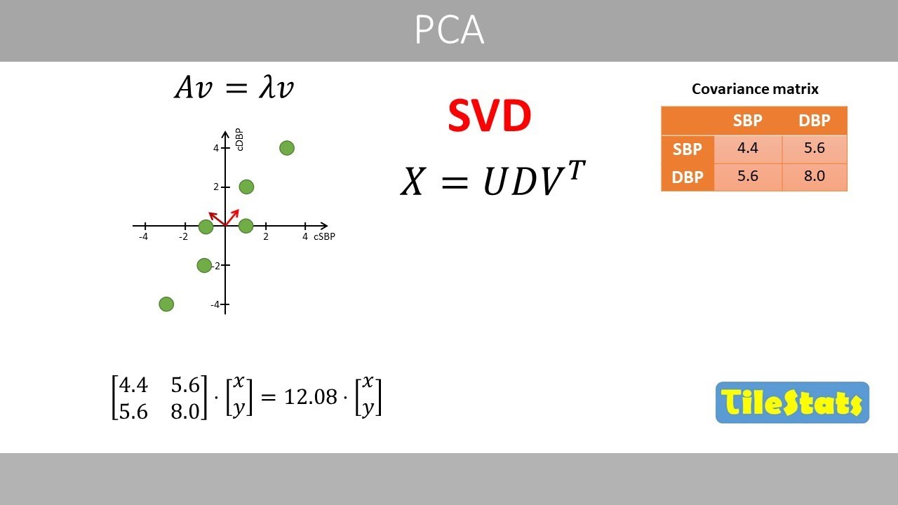
which can be plotted like this.

Next, we calculate the coariance matrix

based on the center data. If you instead

scale or standardize the data, the

covariance matrix will be equal to the

correlation matrix.

Note that the main diagonal of the

coariance matrix includes the variance

of each variable.

The sample variance of the systolic

blood pressure is calculated like this.

When we calculate the variance of the

centered data, the calculations become a

bit simpler since the mean of the

centered data is always equal to zero.

To calculate the sample variance of the

centered data, we therefore simply sum

the squared centered values and divide

by the sample size minus one.

Then we calculate the variance of the

diastolic blood pressure.

Finally, we calculate the co-variance,

which is a measure of how much the two

variables spread together. The sample

co-variance is calculated by multiplying

the centered values of the two

variables.

For example, we multiply the centered

values for person number one and then

add that to the product of the centered

values for person number two and so

forth. Finally, we divide the sum of the

products by the sample size minus one.

We see that the spread in the diastolic

blood pressure is a bit higher than the

spread in the systolic blood pressure.

The co-variance is somewhere between

these two values.

Next, we calculate the igen values of

the covariance matrix.

We substitute a by the co-variance

matrix

and this term by lambda times the

identity matrix which has the same

number of rows and columns as the

covariance matrix.

Subtracting these two matrices results

in the following matrix.

Next we calculate the determinant of

this matrix

which is the product of this diagonal

minus

the product of this diagonal.

After some simplifications

we have the following quadratic

equation. Quadratic equations like this

can be solved in different ways which

will not be discussed here. Anyway, if

you plot how the left hand side changes

as a function of different values of

lambda, we see that the left hand side

is equal to zero when lambda is equal to

either

about 0.32

or 12.08.

These two values represent our values of

the covariance matrix. Next, we

calculate the corresponding vectors to

these two values. We will start by

calculating the igen vector of the

covariance matrix with the corresponding

value 12.08.

To calculate the igen vectors of the

coariance matrix, we use the following

equation that we have discussed in the

previous video about vectors.

We plug in the coariance matrix and one

of the two values. If you multiply the

coarience matrix by this column vector

and multiply the igen value by the same

vector, we'll get the following system

of equations.

We move these two terms to the right

hand side.

After some simplifications, we have the

following system of equations.

Solving for y in the two equations

results in that y is equal to 1.37x.

For example, if you set x equal to 1,

y is equal to 1.37.

This vector is therefore an en vector of

the covariance matrix. We can illustrate

this vector in the plot like this by

drawing an arrow from the origin to the

coordinates

one and 1.37.

We will now normalize this vector to

unit length which means that it should

have a length of one.

The length of this vector is about 1.7.

And if we divide these values by 1.7,

we'll get the igon vector with unit

length.

This vector represents one out of two

vectors of the coariance matrix.

To find the second vector, we do the

same calculations as before based on the

second value. After some calculations,

this vector represents our second vector

with unit length. Since the coariance

matrix is symmetric, its igen vectors

corresponding to distinct values are

orthogonal. Therefore, their angle is

90°.

Next, we order the igen vectors based on

their corresponding igen values where

the igen vector associated with the

largest igen value becomes our first

vector. Since this igen vector is

associated with the largest value, it

will represent our first vector. We

therefore rename this vector so that it

is called v1 instead of v2. Let's put

these two vectors together into a matrix

that we called V. The first column

represents the first vector whereas the

second column represents our second

vector.

We now use this matrix to transform our

center data so that the two variables

are completely uncorrelated.

Let's define our centered data as matrix

X.

Next, we multiply our data matrix X by

matrix V. Then we get a new matrix with

a transformed data. This transformed

data is called principal component

scores or just scores. When we go from

our centered data to the transformed

data, this can be seen as we rotate the

data clockwise until the two en vectors

point in the same direction as the x and

y axis of the plot. The rotated data now

looks like this. Note that the labels of

the axis have now been changed to

principal components one and two.

Let's call the two columns of the

transformed data PC1 and PC2.

If we were to plot this data, we would

get the following plot.

Let's compare the centered data with the

transformed data.

The variance of the systolic blood

pressure is 4.4

whereas the variance of the diastolic

blood pressure is eight.

This is the covariance matrix of the

data. We see that the co-variance is 5.6

which tells us that there is a positive

correlation between the two variables.

When we transform the data, the first

variable called PC1 has a variance of

12.08

whereas PC2 has only a variance of 0.32.

This means that almost all variance is

kept in the first principal component.

If you divide the variance of the first

principal component

by the total variance, we see that the

first principal component captures 97.4%

of the total variance.

Note that the variances of the principal

components correspond to the two values

we calculated earlier. The igen values

of the covariance matrix therefore

represent the variances of the principal

components.

When we study the covariance matrix of

our transform data, we see that the

co-variance between PC1 and PC2 is equal

to zero. Which means that PC1 and PC2

are completely uncorrelated.

Note that the total variance of PC1 and

PC2 is about 12.4 four which corresponds

to the total variance of the original

variables.

Remember that when we multiplied our

centered data by the matrix that

includes the vectors as columns, we got

the transformed data. This is the same

as using the following equation to

calculate the principal components that

we saw at the beginning of this video

where the weights for the first

principal component comes from the first

vector whereas the weights for the

second principal component come from the

second vector. For example, if we would

calculate the corresponding score for

person number six, we would multiply the

centered blood pressure values of person

number six by the corresponding weights.

By adding these products, we would get a

principal component score of five.

Note that the general aim of using PCA

is to reduce the dimensionality of the

data. In other words, we like to reduce

the number of variables we have. But so

far, we have not reduced the number of

variables since we have the same number

of principal components as the number of

variables we started with. Since the

first principal component captures

almost all variance which can be

interpreted as it stores almost all

information about the two variables. We

can simply delete the second principal

component because it includes almost no

information.

As we have seen previously by using the

following equation we can combine the

two variables into just one variable in

a way that maximizes the variance of the

linear combination

we have. so far used the iggon de

composition of the coarience matrix to

compute the PCA. We'll now have a look

at how to compute the principal

component scores by instead using the

singular value de composition.

The SVD method does not involve the

computation of the covariance matrix.

Instead, SVD solves the following

equation which involves numerical

methods so that the product of these

three matrices is as similar as possible

to the data matrix X which is our

centered values.

Solving this equation is generally more

accurate than the igen decomposition

method because it works directly on the

data matrix X without computing the

covariance matrix that may cause

rounding errors. I will not go into all

the details of SVD. Instead, I will try

to explain what this equation means. We

will start by calculating the so-called

grand matrix where we multiply the

transpose of the center data by the

center data which results in the

following matrix.

Note that by multiplying for example the

second column of the center data by the

first row of its transpose

it's exactly the same calculation that

we do in the numerator when we calculate

the covariance between the two

variables.

This means that we will get the

corresponding coariance matrix if we

divide the gram matrix by n minus one.

We'll now compute the igen values of the

grand matrix

which results in the following values.

If we would divide these values by n

minus one, we'll get the exact same

values as when we compute these based on

the covariance matrix. If you now

compute the igen vector based on the

first value,

we will end up with the same vector with

the unit length as we computed based on

the covariance matrix.

So when we compute the igen vectors and

the igen values of the gram matrix

instead of the covariance matrix we get

the same vectors but different values.

We can now create an igen value matrix

of these two values

like this.

Note that when the igen vectors are

multiplied by the igen value matrix and

then multiplied by the transpose of the

igen vectors,

we get the gram matrix.

If you take the square root of these

values,

we will get the so-cal singular values.

The main idea with the SVD method in PCA

is to factoriize a matrix

into three parts

where the rows in their transpose of V,

the vectors tell us how to rotate the

coordinate axis to point in the

directions of maximum variance.

Matrix D tell us how the data stretch

along each of these new axis. Whereas

matrix U tell us where each observation

lies after the rotation before

multiplying by D which may either

stretch or compress the data points

along the new axis. But how do we

calculate matrix U?

Well, the SVD method computes this

numerically. But let's try to do this by

hand. If you multiply both sides by a

matrix V,

this product will result in the identity

matrix because the igen vector matrix is

orthonormal. Next, we multiply both

sides by the inverse of the matrix D

where this product also results in the

identity matrix.

So we now know how to calculate matrix

U.

This is the inverse of matrix D. So if

you multiply matrix X our center data by

the igen vector matrix V and then by the

inverse of matrix D we will get matrix

U.

So this is our certain data. The rows of

the transposed

vector matrix tell us how the data will

be rotated.

Whereas matrix U gives the coordinates

of the data points in their rotated

principal component space before they

are stretched by the singular values in

D. Note that when we multiply these two

matrices,

the xcoordinates of the data points in

the new space are multiplied by 7.77

whereas the ycoordinates of the points

are multiplied by 1.26.

So that this data is stretched out like

this.

So if you multiply matrix U

by matrix D,

we get the final principal component

scores. And if you multiply these by the

transpose of the igen vector matrix,

we will recreate the original center

data points, which is exactly what this

equation tells us.

To compute the final principal component

scores, we may either multiply matrix U

by matrix D

or simply multiply matrix X by the

vector matrix V.

So this is how you would compute the

decomposition in R.

We first create a matrix of our two

variables.

Then we center the data with the

function scale.

If you instead like to scale your data,

you should set this argument to true.

Then we compute the covariance matrix

and the igen vectors of the covariance

matrix. Finally, we multiply the center

data by the igen vector matrix to get

the principal component scores.

We can also use the SVD method by using

the SVD function that will give us the

D, U, and B matrices.

If you multiply the centered data by the

EN vector matrix, we'll get the

principal component scores which are

identical to these scores.

Depending on your data, you might see

some small differences between the

scores of the two methods.

Note that the prome function in R uses

the SVD method and not the en

decomposition.

The corresponding code for computing the

IGEN decomposition in Python can be

written like this.

Note that we here need to sort the igen

vectors so that the first vector is the

one associated with the largest value.

Also note that Python has negative

values for the first vector

which explains why the scores have

opposite signs compared to the example

in this video. To perform PCA with the

SVD method, we can for example use the

PCA class from the skyit learn.

Before we end this lecture, let's try to

understand why the first vector points

in the direction that has maximal

variance.

From our previous calculations, we know

that the first principal component has a

variance of 12.08.

We got these principal component scores

by multiplying the first vector by the

centered values.

So we can define it like this where the

variance of matrix X times the first

vector is 12.08.

From the previous calculations, we know

that the igen value that we computed

based on the covariance matrix is also

12.08.

The variance of the first principal

component is actually equal to the first

value. This is the definition of an igon

vector

where matrix A in PCA is our covariance

matrix which is usually denoted with

this symbol. If you solve this equation

for the value, we will obtain this

equation given that vector V has unit

length. If you plug in the right hand

side here,

we will get this equation.

We want to find a vector V with unit

length that maximizes the variance. If

the length of the vector is equal to

one, the transpose of the vector times

the vector itself should be equal to one

that I showed at the beginning of this

video. When we have a constraint like

this, one method is to use the lrange

multiplier where this term enforces the

values of the vector to fulfill these

conditions.

If we take the derivative of this

equation with respect to v1, we will

obtain the following equation. We now

set the left hand side to zero

because the derivative is equal to zero

when we reach the maximum of this

function.

We can now rearrange this equation and

cancel the twos.

So that we end up with this equation

which is identical to the equation for

the definition of an vector. So this

explains why the first igen vector

points in the direction with maximal

variance. This was the end of this video

about the fundamental math behind PCA.

Thanks for watching.