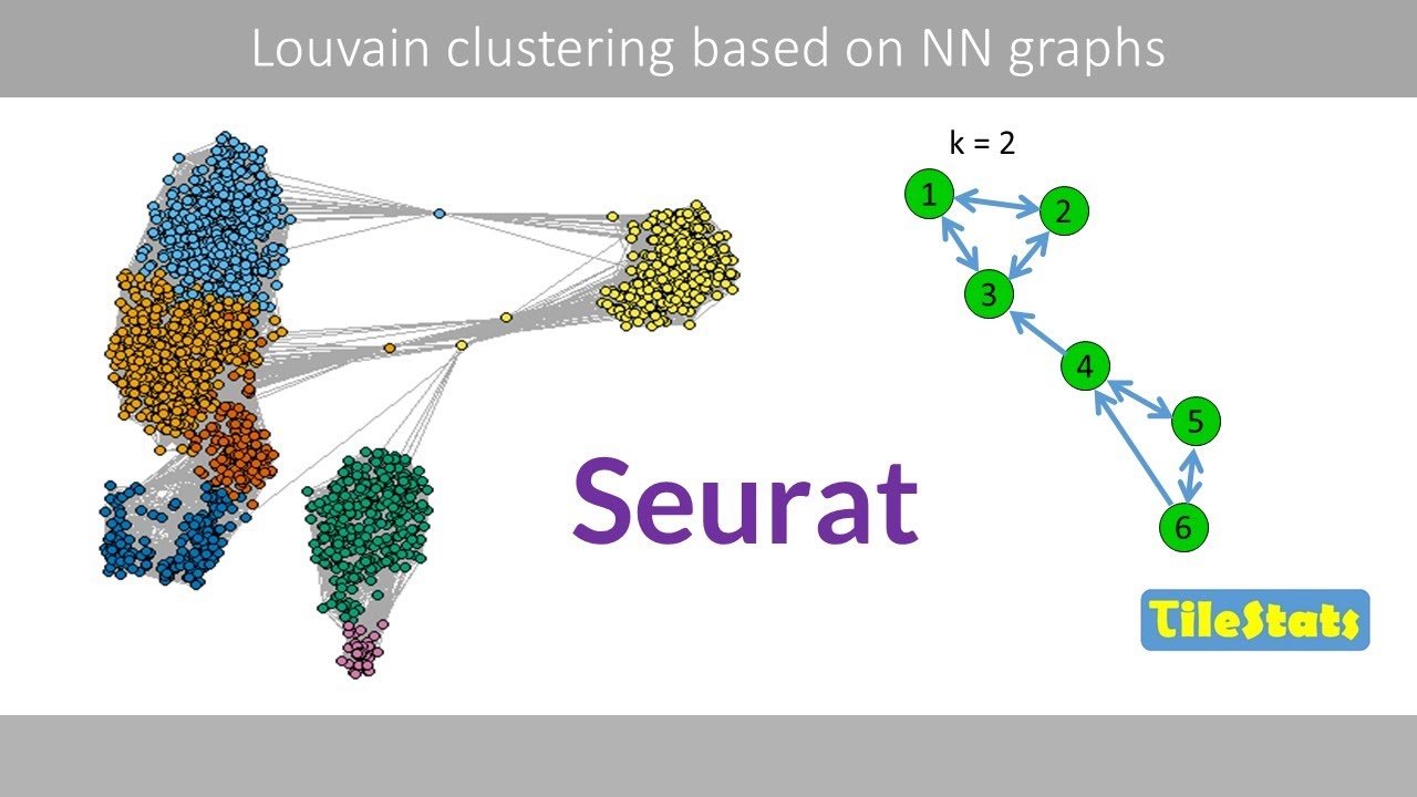
In this video, we'll see how to build

KN&N and SNN graphs and how to identify

clusters in such graphs using the Luain

method similar to what is done in the R

package serat to identify clusters of

cells from single cell RNA seek data. We

will start by creating a K nearest

neighbor graph or a K&N graph based on

some simple data. Note that we may have

data in several dimensions because the

graph is built on distances between the

data points in a multi-dimensional

space. I will here use the cladian

distance as a distance measure. For

example, to calculate the client

distance between data points one and

six,

we plug in their x and y coordinates and

do the math. If we have, for example,

three variables with points in a

three-dimensional space, we would

instead use this equation to calculate

the distance, then we fill in the value

in the distance matrix that shows the

distance between data points one and

six. Then we compute the clarion

distances between all data points so

that we get the following distance

matrix. Next, we determine the number of

closest neighbors a data point should

connect to. As an example, I will here

set this value to two.

So for data point one, we see that its

closest neighbors are data points two

and three. We now create an adjacency

matrix that indicates that data point

one is connected to data points two and

three. So this means that data point one

is connected to

data points two and three but not to the

other data points. We can now start to

draw a directed graph where the arrows

means the data point one is connected to

data points two and three. Next, we see

that data point two has data points one

and three as its closest neighbors,

which means that we add an arrow that

points from two to three and an arrow

that points from two to one.

The two closest neighbors to data point

three are data points one and two, which

means that we add arrows from data point

three to data points one and two. We now

continue to build the graph.

So this is our final CAN graph. Note

that a data point in this graph is

called a node and that the line between

two nodes is called an edge.

Sometimes one also adds edges that point

to the node itself to show that the

point has its closest distance to itself

which means that there will be ones in

the main diagonal in the adjacency

matrix. Anyway, we will not use such

self connections for our graph.

So what we have here is a so-called

directed graph because it includes

arrows that show which data points that

are the closest neighbors for a given

data point. By the arrows we can for

example see the data point four has data

points three and five as its closest

neighbors. One can convert this directed

graph to an undirected graph by simply

removing the arrows from this graph.

like this.

This edge tells us that there is a

connection between points three and

four. But not whether three includes

point 4 as its two closest neighbors.

When we go from a directed graph to an

undirected graph, we need to update the

adjacency matrix. For example, we should

put a one here to define that there is a

link between points three and four

because we know that there is a

connection between these two points.

Same here because there is a connection

between points four and six. So this is

our updated adjacency matrix based on

the undirected graph. Note that this

matrix is symmetric because the elements

in the upper triangle hold the same

values as the ones in the lower

triangle.

We'll now see how to create a simple

weighted CANN graph.

One simple way to put weights on our

graph would be to compute the inverse of

the Eian distances.

For example, the weight between data

points one and two is 1 / 0.14,

which is 7.14.

If we were to compute the inverse of

these distances,

we would run into a problem because we

cannot divide by zero, one therefore

usually replaces the zeros with a very

small value to do such a computation.

Then we simply multiply the recrocal

values by the adjacency matrix element

wise so that we get the weighted

adjacency matrix. We can now fill in the

weights in our graph like this.

A higher value means that we put more

weight on a connection when we interpret

the graph. We'll now see how to build a

shared nearest neighbor graph or an SNN

graph which is for example used in

Serat's single cell RNA seek pipeline to

identify clusters of cells.

An SNN graph starts from a directed KN&N

graph. Then we basically copy the CANN

graph but where we do not include its

directions so that we have an undirected

K&N graph. Note that an SNN graph can be

built in many different ways and this is

only one way to create such a graph. To

create an SNN graph, we add an edge

between all pairwise points that share

at least one neighbor. Since points one

and four share the same neighbor, which

is data point three, we add an edge

between points one and four. And since

data points two and four also share the

same neighbor, we add an edge between

points two and four. For example, 0.5

does not share any neighbors with points

one, two, and three, which means that no

edge is added between these nodes.

So this is our final SN graph. We can

now add weights to this graph. One way

is to compute inverse of the ecclesian

distances that we did before. But I will

here show another method based on the

number of shared nearest neighbors.

Such weights will span between zero and

k + one since the node itself is

included in its own nearest neighbor

set. This means in our case that the

number will span between zero and three.

So for edges that point in both

directions, the weight starts at two and

then we add a one because data points

one and two share one neighbor.

So we fill in this weight here.

We will get the same weights here. Since

this arrow only points in one direction

and that data points three and four do

not share any closest neighbors, this

edge will get the weight one. Since

there is no edge between points one and

four in the cann graph, but they share

one neighbor, the edge will get the

weight one, which is also true for

points two and four.

Since points four and five do not share

any nearest neighbors and have an arrow

that points in both directions, the edge

will get the weight of two.

Since there is one arrow that points in

one direction between points four and

six, and they share one nearest

neighbor, which is five, the edge gets a

weight of two. Finally, the weight

between points five and six is equal to

three because the arrow points in both

directions and they both have 4 as their

closest neighbor. So this is our final

weighted SN graph.

So we have a strong weight here because

points one and two have themselves as

closest neighbors and they share one

neighbor in the directed KN&N graph.

There is a weak weight here because

points two and four were not among their

closest neighbors, but they shared one

neighbor in the director K&N graph. So

these are the same numbers we would get

if we use the function make SNN graph in

the R package bluster by setting type to

number. If you change type from number

to your card,

it will compute the your cardlike

weights based on this equation where n

is number we just calculated and k is

the same k we used previously which was

set to two.

So the yakard weights for these four

edges are equal to one and these three

edges will be equal to 0.2 two whereas

these two edges will get a weight of

0.5.

So this is our weighted SN graph based

on your cardlike indices that span

between zero and one. This graph has

actually the same weights

as I get if I use the function find

neighbors in the seat package version

5.3.0.

However, I was not able to find out the

exact details of how this function

computes the graph and the weights.

Anyway, I got the same graph and the

weights when I tested a range of

different inputs and use different

values of K. So, I assume that they use

the same method. Note that sout includes

the node itself as its closest neighbor

that we discussed previously which means

that we need to set the k parameter to

three and set the ones in the main

diagonal to zero to generate the same sn

graph. Serat also include this

additional pruning parameter which by

default is set to 1 over 15. If you set

this to 0.25 25. In our example, we

would delete these edges because these

edges have weights that are less than

0.25.

So that we have the following prune

graph. I will now briefly show how Lane

clustering can be used to identify

clusters or communities in a graph.

Lane clustering is a graphbased method

that tries to maximize the modularity

score Q which is high when nodes have

many edges inside their cluster and

fewer edges between clusters than

expected by chance.

Suppose that we would calculate the

modularity score given that points 1 2

and three are in one cluster and points

four five and six are in a second

cluster.

So this term will therefore be equal to

one if two nodes i and j are within the

same cluster and zero otherwise.

The sum of the weights for all edges is

in our example equal to five.

For example, the edge weight between

node one and two is one and the sum of

the edge weights for node one is two

which is true also for node two. Based

on this equation, the modularity score

for a certain cluster can be calculated

by the following simplified equation

where sum in is the sum of the edge

weights between nodes within cluster C

where each edge is considered twice. The

sum total is the sum of all edge weights

between nodes within cluster C and also

edges between clusters.

Since nodes in different clusters do not

contribute to the modularity score Q, we

only need to sum the scores for each

cluster to get the final score.

So the modularity score for cluster one

is 0.24

because the sum of the edge weights in

cluster one is three and since each edge

is considered twice, the sum within the

cluster is six. And since no node within

this cluster is connected to nodes in

the other cluster, the total sum is also

six.

The modularity score for the second

cluster is also 0.24.

The sum of these scores is therefore

0.48

which is our final modularity score.

Suppose that there will be an edge

between two nodes in different clusters

that has a weight of one. The modularity

score would then be lower because edges

between clusters will reduce the

modularity score. If we would use this

type of clustering where nodes one and

two are in one cluster and nodes three

to six are in the second cluster, we

will get a much lower modularity score

because edges between clusters will

increase the value in the numerator of

this term which reduces the modularity

score. If you try to use three clusters,

the modularity score is also relatively

low because a cluster with a single node

will get the value of zero for this term

and a negative value here due to its

connections to cluster one which results

in a negative score for this cluster.

And since the nodes in cluster one now

connect to the node in cluster three,

the modularity score is almost zero for

this cluster.

Finally, if you have just one cluster,

the total modularity score is zero

because these two terms are equal to

one. By evaluating all possible

clusters, two clusters with these nodes

will give the highest modularity score.

The leane clustering does therefore not

only put the nodes in the correct

clusters, it also identifies the most

appropriate number of clusters.

However, one can include the so-called

resolution parameter in this equation.

This is a hyperparameter

which is set by the user to adjust the

number of generated clusters. A larger

value of this parameter results in more

clusters whereas a smaller value results

in fewer clusters.

This was the end of this video about

KN&N and SN graphs and Louane

clustering. Thanks for watching.