Today we will discuss the diffusion

model that is used in generative AI to

produce for example images and videos. I

will first explain what diffusion is and

then explain how this equation works to

apply forward diffusion on an image.

This equation is the key to understand

the diffusion model. Next, we will

discuss how a simple neural network can

be trained to learn the added noise from

the forward diffusion and finally see

how the train network can recreate an

image from complete noise by backward

diffusion. I will mainly focus on the

DDPM model that was published in 2020

and show the basic equations from this

paper at the end of this video.

Suppose that we add a drop of ink in

water. The dye molecules in the ink then

start to diffuse and will eventually be

evenly spread out due to the diffusion.

What you see here is a simulation of

diffusion that might represent the

particle that diffuses in a

two-dimensional space. The random

movement of the particle is caused by

collisions with other particles which

make the particle move in a random path.

One way we can simulate such random

movements is to place a point in a

two-dimensional plot. The initial

position of the point is here placed at

an xcoordinate of 10 and a ycoordinate

of 20. Then we draw two random values

from a standard normal or Gaussian

distribution which has a mean of zero

and a standard deviation of one. This

notation tells us that epsilon is

distributed according to a normal

distribution with a mean of zero and a

standard deviation of one. Remember that

the variance is the square of the

standard deviation which means that the

standard normal distribution has also a

variance of one. Suppose that we draw

these two random values from the

distribution.

So to update the x and y positions of

the point, we add the random values to

the current x and y coordinates and do

the math. Then we move the point to the

updated position.

Next, we draw two new random values from

the distribution which happen to be one

and -3.

Note that it is more likely to draw

values between -1 and positive1 from the

normal distribution than values in the

tails.

Then we add these two random values to

the current coordinates and calculate

the new position of the point

and update its coordinates. Then we just

continue like this.

Now let's say that a particle can only

diffuse in one dimension which is here

the x dimension. This means that we now

just draw one random value from the

distribution and add this to the current

xcoordinate.

Then we only need to update its position

in X since the Y-coordinate is fixed.

Then we draw a new random value and

update its position and so forth. To

easier track the trajectory path over

time in one dimension, let's put the X

coordinate on the Y axis and T for time

on the Xaxis.

So at time point Z the initial position

of the point is 10. Then we draw a

random value from the standard normal

distribution and add that to the current

position

which means that the x position for the

next time point is 8. Then we draw a new

random value and update the current x

position and so forth.

If you simulate for 500 time steps, the

trajectory of the X position over time

might look something like this. Note

that every time we simulate, we will get

a different trajectory due to the

stochastic process. The distribution of

the X values can be illustrated by the

following histogram. We see that the x

values span between 0 and 45

which corresponds to the range in this

plot.

If instead simulate 5,000 time steps,

the distribution now becomes wider. The

values now span between80

and positive40.

So the variance increases with time for

this kind of process. However, in

diffusion models, we like to have the

following diffusion process.

I've here started at 100 so that we

clearly can see how the signal goes down

to zero. This initial signal may

represent a pixel value in an image.

So, every plot like this may represent

the value in a pixel over time. Each

pixel will have its own random

trajectory.

We want that the signal or the value in

the pixel to go down to zero where the

variance of the noise should stabilize

around one

because the image then contains pure

noise.

So this pixel may have a value of 100

that represents white color. After some

time the pixel may have a value of zero

which represents gray color. This

process is called forward diffusion

because we add noise in the image over

time. This is an example of forward

diffusion in a real image.

After some time the image will contain

pure noise.

The distribution of the noise after

about 2,000 time steps reflects the

normal distribution with a mean of zero

and a variance of one

to generate this type of noisy curve.

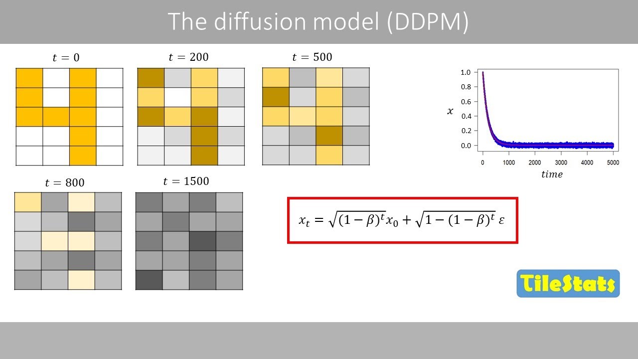
We can use the following equation to

simplify things. I will here use a fixed

value of beta. But in diffusion models,

beta is varied over time. In the DDPM

model, beta increases linearly over

time. Note that the value of beta should

always be somewhere between zero and

one.

If you plug in our fixed value of beta

and simplify,

we see that the previous x value will be

multiplied by a value that is smaller

than one. which means that the

subsequent x values will approach zero.

One can see this as we remove 0.5%

of the signal at each time step. If you

compute the product of 1,000 of these

values

and multiply with the initial signal, we

see that the initial signal has been

reduced close to zero after 1,000 time

steps. After 2,000 time steps, the

initial signal is very close to zero,

which means that the signal in the image

has been almost completely lost and that

the image now contains pure noise. In a

diffusion model, we like to train a

neural network to predict a specific

noise sample drawn from a normal

distribution that was added to the

current x value.

So for training we do not need the full

trajectory over time. We only need the

current x value and the added noise at

this time point because the network can

then predict the added noise at the

given time point. If you generate 1,000

of these random trajectories, we can see

how they have spread out. If you plot

the 1,000 values at time point 5,000, we

see that they are normally distributed

with a mean of zero and a variance of

one. If you delete this term, we can

plot how the signal decays over time

without the noise.

We can see that the signal has gone down

to zero after enough time steps. Instead

of creating many trajectories like this,

we can generate similar random values

around the curve with the following

closed form formula assuming a fixed

value of beta.

Note that we here use only the initial

value of x instead of iterating over

time.

If you set t to for example 5,000, we

can compute a random value around the

curve directly without the need to

iterate until we reach that time step

because this equation depends only on

the initial value and the current time

point. If you plug in the value of beta

which is here assumed to be fixed and

simplified we see that if time goes to

infinity

this term will go to zero whereas this

term will be equal to one.

This explains why we have pure Gaussian

noise with a mean of zero and a variance

of one after many time steps because the

forward diffusion has eliminated the

information about the initial signal.

The initial value of x

when t is small the value of x for the

next time step will depend a lot on the

initial signal where very little noise

is added because this term will be

almost zero for small t's. The variance

of the noise added at the given time

point can be defined like this. And the

standard deviation of the added noise is

therefore the square root of the

variance. For example, the variance of

the noise that is added at time 20 is

about 0.18.

about 0.95

of the 300 time steps and about one of

the 1,000 time steps.

Note that in diffusion models, beta is

allowed to change during the forward

diffusion. In the DDPM model, beta

starts with a small value which is

increased for each time step.

This means that we need to compute the

cumulative product for the current time

point. Instead of simply taking 1 minus

beta to the power of t. If we use the

cumulative product, we use instead this

equation for the forward diffusion. I

will come back to this equation at the

end of this video when we have a look at

the DDPM paper. Anyway, since we use a

fixed value of beta, we can use a

simpler form of the equation.

A reduced value of beta means that it

will take longer time to reach pure

noise.

Now, let's see how we can train a simple

neural network.

I will here use a super simple neural

network without any hidden layers and

with a linear activation function. Note

that this network is way too simple to

learn the forward diffusion, but it will

help us to understand the basics.

As input, the network takes the value of

X at the random time point and the time

at that time point.

It then uses these inputs to predict the

noise that was added at this time point.

The two weights and the bias weight will

now be updated by the method of gradient

descent. To minimize this loss function,

which is the square difference between

the predicted noise and the true noise,

let's use some numbers to understand

this better.

During training, a random time point is

selected. To select a random time point

in this example, we draw a random

integer from a uniform distribution

between 1 and 5,000. This means that

every time point is equally likely to be

selected. In this case, the time point

2,00 was randomly selected. Note that

the time points are usually normalized

so that the values span between zero and

one. But to keep things simple, we here

use the raw time points. This time point

is now plugged into this equation

together with a random value drawn from

a normal distribution with a mean of

zero and a variance of one.

Suppose that this value happens to be

0.5.

The computed value of X is therefore

about 0.504

at the time point 2000

because we still have some small signal

left at this time point.

This value can be seen as we pick a

random value around the curve at the

time point 2000.

We now plug in the value of x and the

value of t as inputs in the network.

Now suppose that the current values of

the weights are equal to these values.

If you plug in these weights and the

input values, we see that the network

predicts the added noise to about 0.8.

We can now calculate the loss where we

plug in the true noise that was added

and the predicted noise by the network.

We see that the loss is 0.09.

Now the network will try to reduce this

loss by updating the values of these

weights with the method of gradient

descent.

A new random time point is then selected

and the network then predicts the added

noise at this time point and updates its

weights to reduce the loss function.

This process will be repeated thousands

of times.

Once the network has been trained, we

will use the train network to perform

backward diffusion.

To perform backward diffusion, we start

at the final time step where we have

pure noise. Since the train network has

now optimized these weights, the values

of these weights will be fixed during

the backward diffusion.

We know that the signal is zero at this

time step and that the noise has a

variance of one.

The initial value for the backward

diffusion process can therefore be drawn

from a normal distribution with a mean

of zero and a variance of one. It is

therefore important that we run the

forward diffusion long enough to make

sure that the signal is close to zero so

that the backward diffusion can be

initialized by drawing a value from a

normal distribution with a mean of zero.

For example, suppose that this value

would be 0.3.

We now plug in the value of XT

and the current time point in the input

nodes.

Let's assume that the network predicts

that the added noise at this time point

was 0.4.

We can now use the following equation to

compute the backward diffusion. If you

use a fixed value of beta, one can

interpret this equation as it removes

the predicted noise

from the signal at time t so that we

predict the signal without the noise one

time step backward in time.

These terms can be seen as scaling

factors that are used so that the

backward diffusion reflects the forward

diffusion.

But why do we use this term?

Zed is actually a random value drawn

from a normal distribution. The reason

why we add new noise in the backward

diffusion process is that the network

was trained to predict the noise during

the forward diffusion and it must

therefore receive a similar type of data

as it was trained on. Also by adding new

noise we will end up with different

values of X0 every time we use backward

diffusion which produces slightly

different images and therefore results

in different outputs from the same

trained model.

Let's plug in our numbers

and do the math.

We now plug in this as input to the

network which predicts the noise that we

plug in here. We update the current time

point and the current value of X and

draw a new random value

and calculate the predicted value of X

at time point 4,998

that we plug in here. We then continue

to iterate like this until we end up

with a predicted value of x at time

point zero which should be close to the

initial signal. Note that in the last

time step of the iteration when we

compute x0 we do not add any noise.

So when we apply backward diffusion on

the real image it may look like this.

To explain how all this works for image

generation, let's assume that we have

the following image with 20 pixels that

is supposed to represent the digit four.

Each pixel in this image holds a certain

normalized value. In this case, the

white color is displayed in the image if

the pixel value is equal to one. Whereas

a black color is shown if the pixel

value is equal to -1.

We now apply forward diffusion to this

image. Each pixel with white color will

start at the value one and decay down to

zero. Whereas the pixels with black

color start at -1 and increase up to

zero. After about 200 time steps, the

pixels with white color have changed

value from one to about 0.8, which means

that the color has changed towards a

light gray color.

A pixel with black color has changed

value from -1 to about0.8,

which means that it has a dark gray

color. After about 500 time steps, the

image might look something like this.

After about 800 time steps, we can

barely see the original signal. And

after about 1,500 time steps, the image

contains just noise, which is expected

because the forward diffusion is now in

the phase with pure noise.

Once we have trained the network, we can

use it to perform backward diffusion

where we start with an image with pure

noise

and move backward in time

until we reach the time of zero. Note

that this image will probably not look

like the original image because noise is

added in the backward process.

The type of network that is used in

diffusion models is usually a so-called

unit that I have explained in a previous

video.

A unit is commonly used for image

segmentation where it can take for

example a satellite image to generate a

segmented image that identifies roads,

lakes, and houses.

In diffusion models, the input in the

unit during training is instead the

image at the certain time point. The

unit also integrates the current time

point in its training.

Some noise has been added to the pixels

in the image at this time point and the

initial values in the pixels have been

reduced down to zero due to the forward

diffusion where the unit tries to

predict the added noise at this time

point which is compared to the true

noise that was added to compute the

loss. The network then updates its

weights that are used during the down

and up sampling to minimize the loss.

Once the unit has been trained, it can

take an image with pure noise and

predict the added noise which is removed

from the current image where also some

new noise is added.

This new image is then used as input to

move backward in time

until it reaches the time of zero.

Okay, let's see if you now can

understand the basic things in a DDPM

paper. On page five, we can see that

they have used 1,000 time steps for the

forward diffusion

and that beta starts at 0.00001

and ends at 0.02 at the last time step.

We can also see that they used a unit.

On page two, they show that alpha t is

the cumulative product of 1 minus beta t

up to the given time point, which is

similar to the equation that I showed

previously.

Since the value of beta is not fixed,

they use this equation for the forward

diffusion.

But what does this equation mean?

Well, this denotes the probability

distribution of X at time t given the

value of x0 which is equal to a normal

distribution of x for a certain time

point which has a mean that is equal to

the original signal multiplied by the

square root of alpha t and a variance

equal to 1 minus alpha t which is

similar to the equation that I showed

previously but where we used a fixed

value of beta for simplicity.

I is just an identity matrix which

indicates that the noise is independent

in each pixel.

On page four, we see that the pixel

values in the image that usually span

between 0 and 255 were scaled so that

the values span between -1 and one.

Similar to our previous example,

if we move to the table on page four, we

can find the training procedure.

So we start by randomly selecting an

image from our data set where X0 is the

normalized pixel values in that image.

Then we draw a random time point based

on a uniform distribution which means

that all time points are equally likely

to be selected. Then we draw random

values one for each pixel in the image

from a normal distribution with a mean

of zero and a variance of one which is

the added noise in the forward diffusion

process.

Next, we compute the square difference

between the added noise and the

predicted noise by the network, which is

computed based on its current weights

and the inputs XT and a time point t

to compute the loss function. These

steps are repeated over all images in a

data set for several epochs until the

network converges where the loss has

stopped decreasing.

Once we have trained the network, we can

use backward diffusion to generate an

image. The initial values in the pixels

at the last time point are drawn from a

normal distribution with a mean of zero

and a variance of one. Then we go

backward from the last time point

stepwise to time point one. When t is

equal to one, we will compute x0.

In each step, we draw random values that

will be added to the pixels as long as t

is greater than one. No noise will be

added in the final step when we compute

x0.

In each iteration, we compute X or the

pixel values one step backward in time.

Sigma T was computed like this. Once we

have ended the loop, we will have our

final AI generated image.

This was the end of this video about the

basics of diffusion models. Thanks for

watching.